Curriculum Learning by Dynamic Instantaneous Hardness
Notes
- Code is available here
Highlights
- This paper proposes a new difficulty metric for curriculum learning called Dynamic Instantaneous Hardness (DIH).
- Its purpose is to speed-up learning and to improve the results.
- It is only tested on classification but might be extended to other applications.
Introduction
Curriculum learning1 consists in presenting the right examples in the right order at the right time during training to enhance the learning process, just as teachers would do with their students. To that end, it is necessary to define a concept of hardness. It can be related to the different classes -in the case of classification- or inherent to the examples, such as specific shapes. One approach, called self-paced learning2, selects some examples at each epoch based on instantaneous feedback from the model. However, it does not take into account the training history of each sample, motivating the introduction of DIH.
Methods
Dynamic Instantaneous Hardness
The goal of the measure is to get the usefulness of each sample in the future in order to select them wisely. The Dynamic Instantaneous Hardness (DIH) is defined as the exponential moving average of instantaneous hardness measures of a sample over time, the instantaneous hardness \(a_t(i)\) being a measure retrieved from the epoch that has just been computed.
\[r_{t+1}(i) = \left\{ \begin{array} 1 \gamma*a_t(i) + (1-\gamma)*r_{t}(i) \quad if \quad i \in S_t \\ r_t(i) \quad else \end{array} \right.\]\(\gamma \in [0,1]\) is a discount factor and \(S_t\) is the set of samples used for training at time \(t\).
Three definitions of instantaneous hardness are compared:
- the loss : \(l(y_i,F(x_i; w_t))\), where \(l(·, ·)\) is a standard loss function and \(F(·; w)\) is the model where \(w\) are the model parameters
- the loss change between two consecutive time steps : \(\|l(y_i,F(x_i; w_t))-l(y_i,F(x_i; w_{t-1}))\|\)
- the prediction flip (the 0-1 indicator of whether the prediction correctness changes) between two consecutive time steps : \(\| 𝟙[\hat{y}^t_i = y_i]- 𝟙[\hat{y}^{t-1}_i = y_i]\|\), where \(\hat{y}^t_i\) is the prediction of sample \(i\) in step \(t\), e.g., \(\arg\max_j F(x_i; w_t)[j]\) for classification.
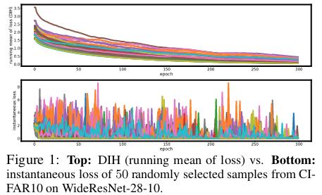
Compared to DIH, instantaneous hardness is i) much less stable during training and ii) requires extra training and inference steps by a model over all the samples.
Properties
DIH can vary a lot between different samples, helping to discriminate between them to select the most informative samples. When it is smaller, the samples are more memorable, i.e. easy to learn, while a larger DIH means that the samples are harder to retain.
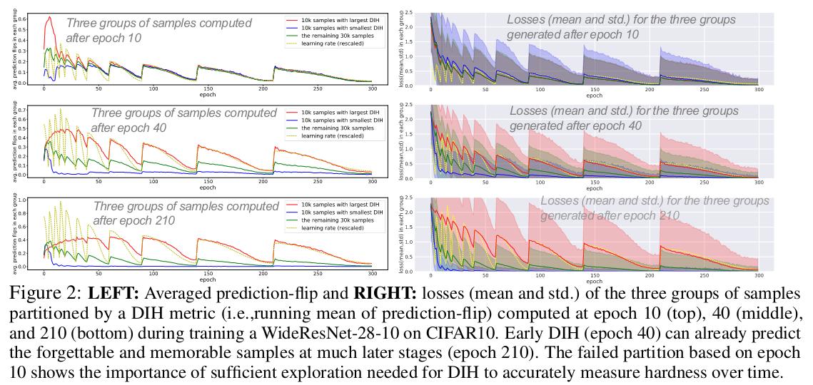 The large steps in the curves are explained by a cyclic learning rate. We clearly see the gap between the training dynamics of red samples that are harder and blue samples that have smaller DIH. Moreover, the variance of loss of samples with larger DIH is bigger showing that a local minima is not found for them. It is thus necessary to revisit them often. The prediction flip leads to the same conclusion; it is higher for the samples that need to be revisited.
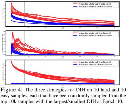
DIH in early epochs (40) suffices to differentiate between easy and hard samples. It doesn’t require a full training to classify the samples. DIH metrics decrease during training for both easy and hard samples, indicating that as learning progresses samples become less informative, and resulting in fewer samples being needed to continue training the model.
Experiments
Curriculum learning
Since the DIH represents the hardness of samples, it seems natural to base some curriculum learning on it (DIHCL). The authors keep training the model on samples whith large DIH that have historically been hard, since the model does not perform well on them, and revisit easy samples less frequently, because the model is more likely to stay at those samples’ minima. At each training step, a subset of samples is selected according to their DIH values, given the probability \(p_{t,i} \propto h(r_{t-1}(i))\), where \(h(·)\) is a monotone non-decreasing function.
- DIHCL-Rand: data is sampled proportionally to DIH \(h(r_t(i)) = r_t(i)\)
- DIHCL-Exp: trade-off between exploration/exploitation based on softmax value \(h(r_t(i)) = exp [\sqrt{2*log(n/n)}*r_t(i)], a_t(i) \leftarrow a_t(i)/p_{t,i} \forall i \in S_t\)
- DIHCL-Beta: Beta prior distribution to balance exploration and exploitation \(h(r_t(i)) \leftarrow Beta(r_t(i),c-r_t(i))\) with \(c > r_t(i)\)
The DIH of selected samples is updated with their instantaneous hardness normalized by the learning rate as it varies during training. During the first few epochs, the whole dataset is used to set a correct DIH for each samples. Once the training starts to select samples, the subset size is gradually decreased during training (empirical study made to find optimal parameters).
Comparison is made with random baseline, SPL (based on instantaneous hardness) and MCL (Minmax curriculum learning3).
Results
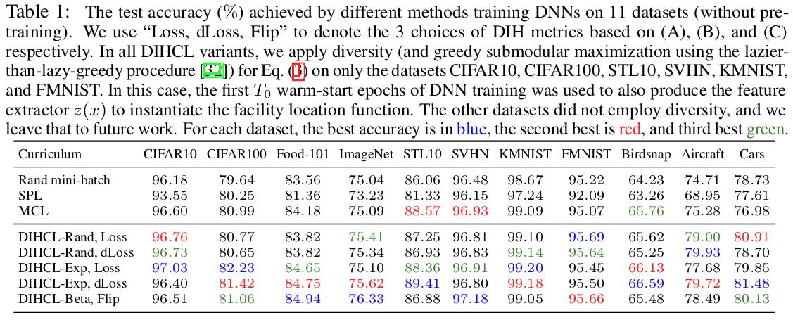
Better accuracy with DIHCL.
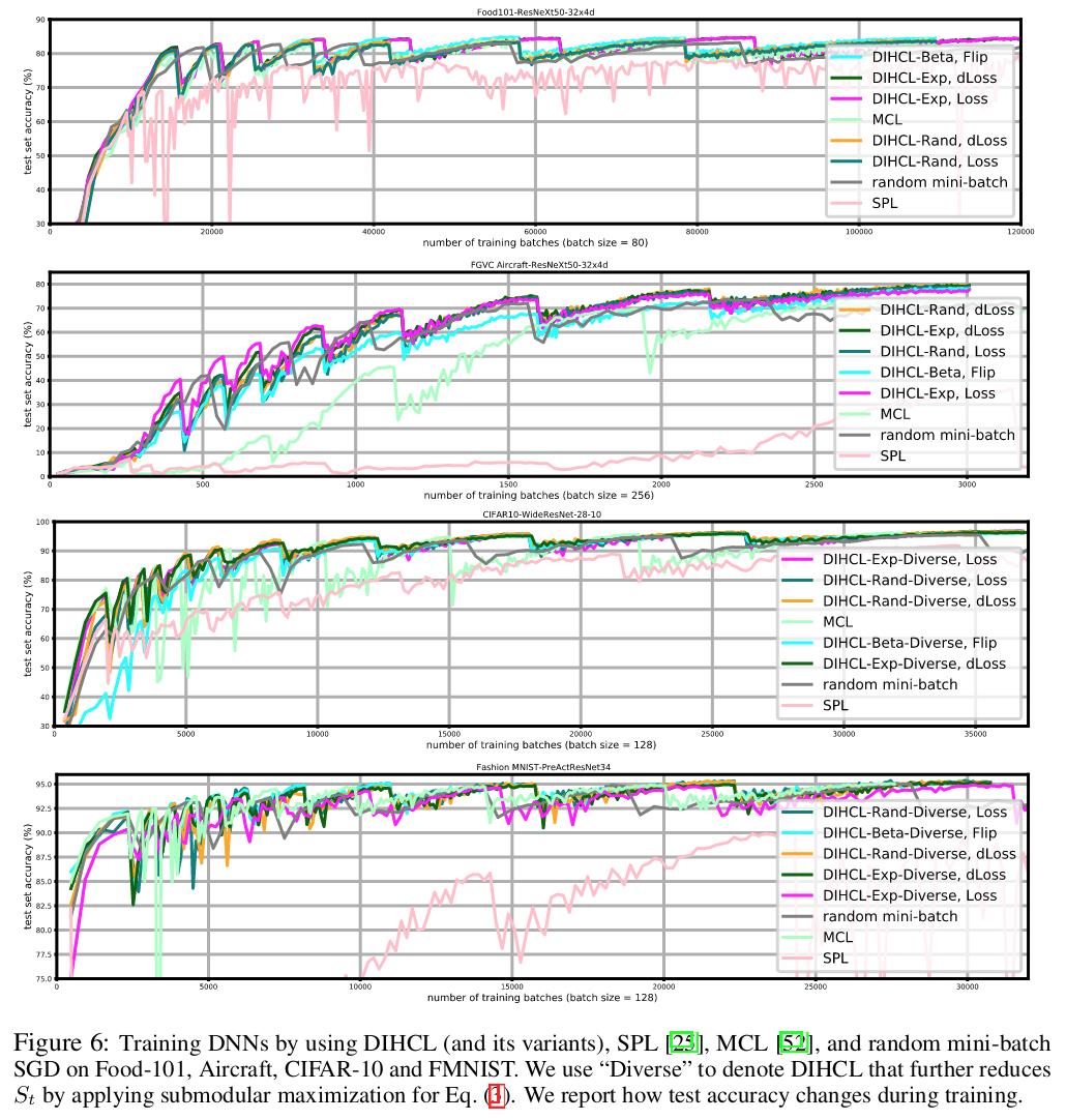
DIHCL is more stable and reaches its best performance sooner than SPL and MCL.
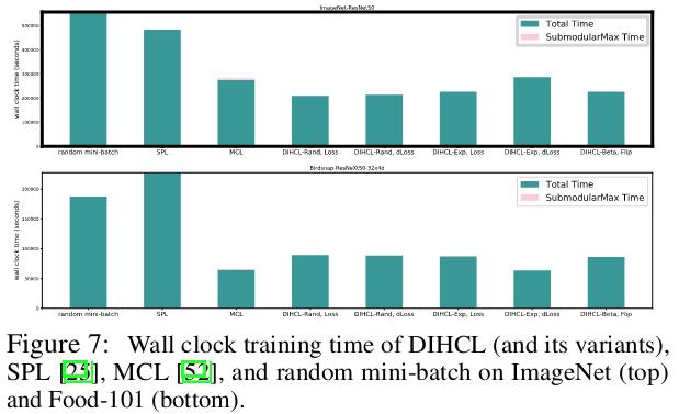
Training time reduced with DIHCL.
Ablation studies

More experiments are presented in the appendix of the article to explain the choice of parameters. The most important settings concern i) the discount factor \(\gamma\) to calculate the DIH, ii) the number of warm starting epochs and iii) the cosine for the cyclic learning rate.
Conclusions
The article introduces a new metric to implement curriculum learning that is doubly benefic as it reduces the training time and does not need a previous training to be set. It would be interesting to compare the performance of DIH to other SOTA CL methods, such as teacher-student CL, aside from SPL and MCL.
References
-
Y. Bengio et al. Curriculum learning. Journal of the American Podiatry Association 60(1):6. January 2009. ↩
-
M. Kumar et al. Self-Paced Learning for Latent Variable Models. Procedings of the 23rd conference on Neural Information Processing Systems. 2010. ↩
-
T. Zhou and J. Bilmes. Minimax curriculum learning: Machine teaching with desirable difficulties and scheduled diversity. In ICLR. February 2018. ↩