Highlights

A new method to generate a heatmap over the input image w.r.t. the pixels’ importance for the prediction, which extends the previous Layer-wise Relevance Propagation (LRP) method to work with negative values.

Introduction

Current techniques to interpret transformers’ predictions suffer from various issues:

Limited to specific subsets of operations/layers allowed (e.g. no negative values);
Simplistic assumptions (e.g. linear combination of attention across network) regarding attention computation;
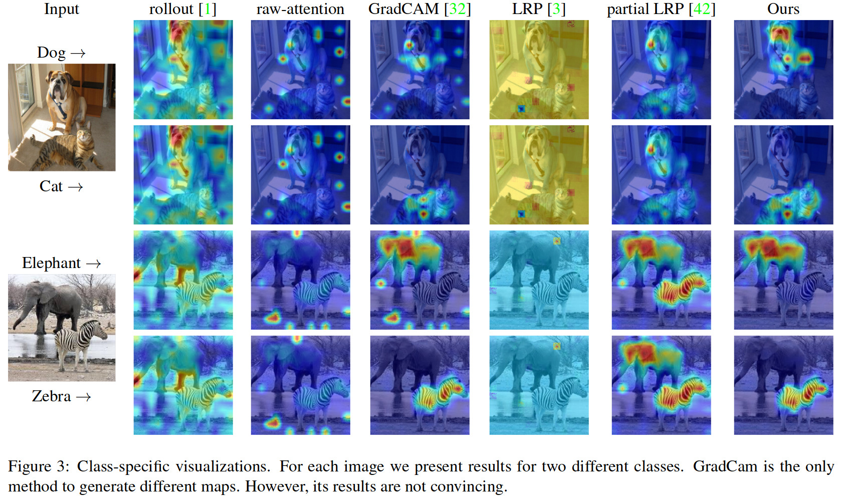
Methods are class-agnostic in practice, meaning their output won’t really change depending on the class, even for methods which in theory take into account class information.

Methods

The method proposed by the authors falls under the umbrella of attribution propagation methods, which are justified theoretically by the Deep Taylor Decomposition (DTD) framework.

To compute the relevance to propagate, the method requires access to the gradients w.r.t. to the classifier’s output \(y\) at class \(t\) (where \(t\) need not be the final prediction of the network).

They denote by \(L^{(n)}(\mathbf{X}, \mathbf{W})\) the layer’s operation on 2 tensors \(\mathbf{X}\) and \(\mathbf{W}\), which typically correspond to the input and weights of the layer (but can also be used for non parametric layers with 2 feature map tensors, such as skip connections).

Given that, the relevance of a layer can (recursively) be defined as:

\[\begin{align} R^{(n)}_j & = \mathcal{G}(\mathbf{X}, \mathbf{W}, R^{(n-1)}) \\ & = \sum_i \mathbf{X}_j \frac{\partial L^{(n)}_i (\mathbf{X}, \mathbf{W})}{\partial \mathbf{X}_j} \frac{R^{(n-1)}_i}{L^{(n)}_i (\mathbf{X}, \mathbf{W})}, \end{align} \tag{1}\]

where indices \(i\) and \(j\) correspond to elements in \(R^{(n)}\) and \(R^{(n-1)}\), respectively, and which satisfies the conservation rule:

\[\sum_j R^{(n)}_j = \sum_i R^{(n-1)}_i. \tag{2}\]

In previous papers, the relevance propagation rule was defined in a way assumed positive values from ReLU activations. Here, the authors propose a definition that generalizes to other activations that output negative values as well as positive ones, such as GELU. They do this by explicitly defining a subset of indices \(q=\{ (i,j) | x_j w_{ji} \ge 0 \}\) that corresponds to positive weighted relevance:

\[\begin{align} R^{(n)}_j & = \mathcal{G}_q(x,w,q,R^{(n-1)}) \\ & = \sum_{ \{ i | (i,j) \in q \} } \frac{x_j w_{ji}}{ \sum_{ \{ j' | (j',i) \in q \} } x_{j'} w_{j'i} } R^{(n-1)}_i \end{align} \tag{3}\]

To initialize the relevance propagation, the relevance in the output layer, i.e \(R^{(0)}\), is set to a one-hot encoding of the class w.r.t. which the relevance should be computed. Starting from there, the relevance can be backpropagated (along with the gradient) through the network.

Numerical instabilities

For the interpretation of the relevance to be useful, the values should remain somewhat bounded. In most layers, this property is implicitly derived from the conservation rule, which dictates that the sum of the relevance in a layer is equal to the sum of the relevance in the previous layer.

However, in some layers, this rule either doesn’t hold up (i.e. matrix multiplications) or is not sufficient in itself to constrain values to remain interpretable because of numerical instabilities which lead to highly positive/negative relevance (i.e. skip connections).

Therefore, the authors propose to normalize the relevance of the 2 tensors such that:

It maintains the conservation rule, i.e. \(\sum_j \bar{R}^{u^{(n)}}_j + \sum_k \bar{R}^{v^{(n)}}_k = \sum_i R^{(n-1)}_i\)
The total relevance for each layer equals 1, i.e. \(\sum_i R^{(n)}_i = 1\)
The relevance sum of each tensor is greater than 0, i.e. \(0 \le \sum_j \bar{R}^{u^{(n)}}_j , \sum_k \bar{R}^{v^{(n)}}_k \le \sum_i R^{(n-1)}_i\)

Final output

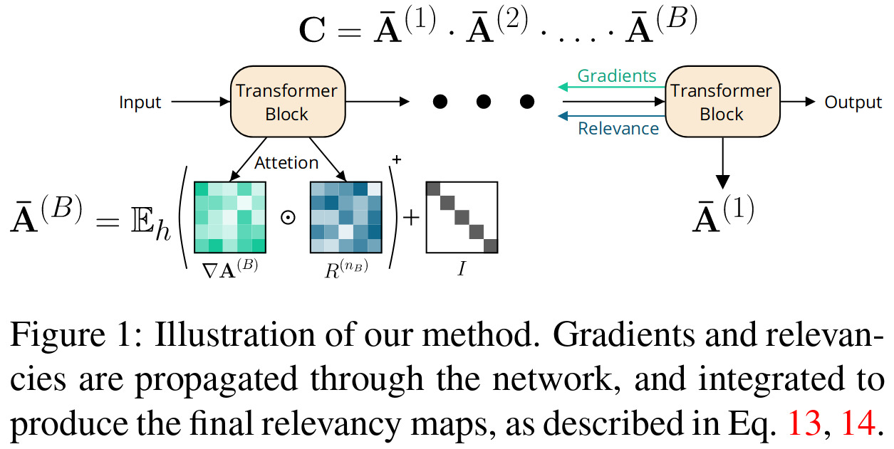
For the specific case of the transformer architecture, given \(\mathbf{A}^{(b)} \in \mathbb{R}^{h \times s \times s}\) the attention map of block \(b\), the propagation of the relevance and the final output \(C \in \mathbb{R}^{s \times s}\) can be defined by the weighted attention relevance:

\[\begin{align} \mathbf{\bar{A}}^{(b)} & = \mathbf{I} + \mathbb{E}_h ( \nabla \mathbf{A}^{(b)} \odot R^{(n_b)} )^+ \tag{4} \\ \mathbf{C} & = \mathbf{\bar{A}}^{(1)} \cdot \mathbf{\bar{A}}^{(2)} \cdot \ldots \cdot \mathbf{\bar{A}}^{(B)} \tag{5} \end{align}\]

The identity matrix in the computation of the propagation of the relevance is there to account for the skip connections and to avoid “self inhibition” for each token.

For comparison, the authors define attention rollout¹ given the same notation:

\[\begin{align} \mathbf{\hat{A}}^{(b)} & = \mathbf{I} + \mathbb{E}_h \mathbf{A}^{(b)} \tag{6} \\ \text{rollout} & = \mathbf{\hat{A}}^{(1)} \cdot \mathbf{\hat{A}}^{(2)} \cdot \ldots \cdot \mathbf{\hat{A}}^{(B)} \tag{7} \end{align}\]

Data

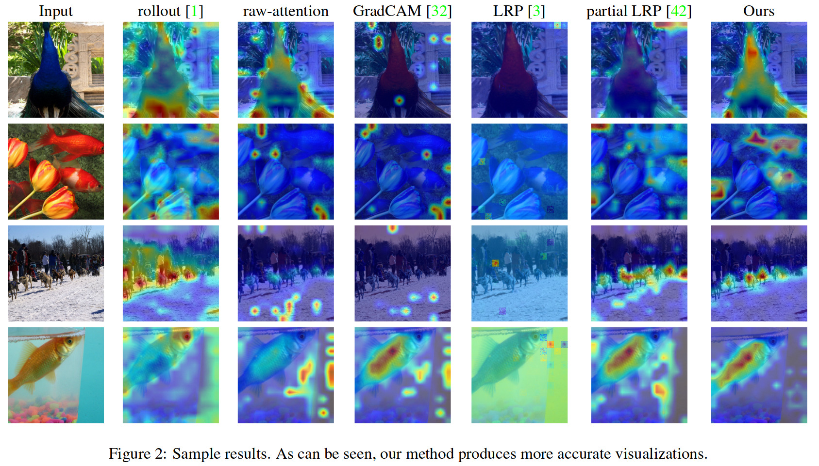
The authors test their method on a vision task (segmentation of ImageNet-segmentation by thresholding the relevance maps by the mean value) and an NLP task (extraction of rationales supporting the binary sentiment classification on the Movie Reviews Dataset). Here we will focus on analyzing the results of the vision task.

Results

Ablation study

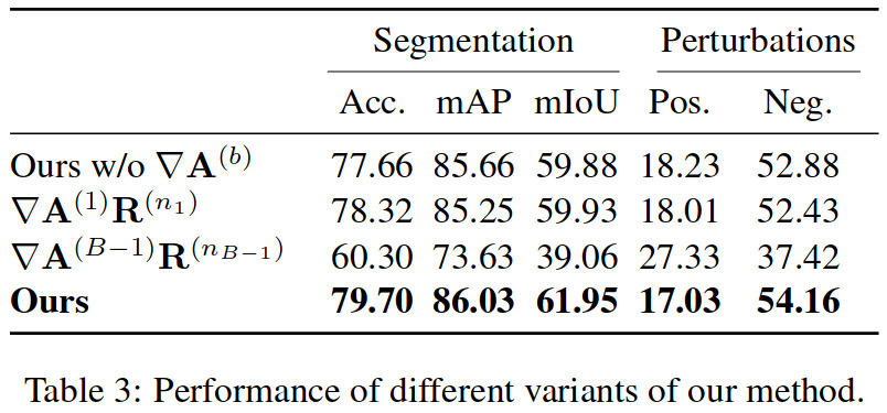
To justify the complete definition of \(C\), the authors perform an ablation study where they evaluate three variants of their method:

Ours w/o \(\nabla \mathbf{A}^{(b)}\): In the definition of the rollout in Eq. 4, use \(\mathbf{A}^{(b)}\), i.e. the raw attention, instead of \(\nabla \mathbf{A}^{(b)}\), i.e. the gradient of the attention;
\(\nabla \mathbf{A}^{(1)} \mathbf{R}^{(n_1)}\): Disregard rollout and use the method only on the last transformer block;
\(\nabla \mathbf{A}^{(B-1)} \mathbf{R}^{(n_{B-1})}\): Disregard rollout and use the method only on the first transformer block.

References

Review of Attention Rollout: https://creatis-myriad.github.io/2022/07/07/AttentionRollout.html ↩