Introduction

In segmentation, it is not always obvious what the correct solution is. Especially in medical image segmentation, experts can disagree about the objects’ boundaries. Ideally this uncertainty about the object boundaries should be captured by the model.

Uncertainty can be divided into two categories:

Aleatoric uncertainty which is inherent to the observations
Epistemic uncertainty which is inherent to the model

In segmentation, aleatoric uncertainty varies spatially i.e. an image can have both regions with higher and lower uncertainty.

The ideal model should represent the joint probability distribution of the labels at every pixel given the image, enabling sampling multiple plausible label maps

Aleatoric uncertainty is inherent to the data and thus can not be reduced. So it is of high interest to model it in sensitive applications. Currently deep-learning methods output only one plausible segmentation with no information on uncertainty. In principle, FCNNs are probabilistic models, since their output is a set of independent categorical distributions per pixel, parameterised by a softmax layer. Because these distributions are independent given the last layer’s activations, sampling from this model would result in spatially incoherent segmentations (grainy label noise in the uncertain regions).

In this context, this paper introduces stochastic segmentation networks (SSNs), a probabilistic method for modeling aleatoric uncertainty that can be easily plugged into any segmentation network. SSNs model joint distributions over entire label maps and thus can generate multiple spatially coherent hypotheses for a single image.

Background

We consider an image \(x\) with \(K\) channels and \(S\) pixels, which maps to a one-hot label map of the same size, \(y\) with \(C\) classes : \(x_i \in \mathbb{R}^K\) and \(y_i \in \{ 0, 1 \} ^C\) for \(i \in \{1,...,S \}\).

In a standard CNN, the probability of one label \(p(y_i \vert x)\) is given by the output of a softmax layer taking in input the logit \(\eta_i\).

Before any independence assumptions, the negative log-likelihood can be written as:

\[- log \ p(y \vert x) = - log \int p(y \vert \eta)p_\theta(\eta \vert x)d\eta \qquad(1)\]

where \(p_\theta(\eta \vert x)\) is the probability of the logit map \(\eta\) given the image \(x\).

Usually we assume that the logit map is given by a deterministic function (our model), \(\eta = f_\theta(x)\).

So \(p_\theta(\eta \vert x)\) can be written as:

\[p_\theta(\eta \vert x) = \delta_{f_\theta(x)}(\eta) \qquad(2)\]

So if we use equation (2) into equation (1) we have :

\[- log \int p(y \vert \eta)p_\theta(\eta \vert x)d\eta = - log \int p(y \vert \eta)\delta_{f_\theta(x)}(\eta) d\eta = - log \ p(y \vert \eta) \qquad(3)\]

The second assumption is that labels \(y_i\) are independent of each others and that each label \(y_i\) only depends on its respective logit \(\eta_i\) :

\[p(y \vert \eta) = \prod_{i=1}^Sp(y_i \vert \eta) = \prod_{i=1}^Sp(y_i \vert \eta_i) \qquad (4)\]

By using (4) into equation (3) and substituting \(p(y_i \vert \eta_i)\) by the output of the softmax layer we get the cross-entropy :

\[- log \ p(y \vert \eta) = - log \prod_{i=1}^Sp(y_i \vert \eta_i) = - log \prod_{i=1}^S \prod_{c=1}^C (softmax( \eta_i )_c)^{y_{ic}} = - \sum_{i=1}^S \sum_{c=1}^C y_{ic} \ log \ softmax( \eta_i )_c \qquad (5)\]

Stochastic Segmentation Networks

In this paper, the authors propose using weaker independence assumptions by using a more expressive distribution over logits. They use a multivariate normal distribution whose parameters are learned by the neural network:

\[\eta \vert x \sim \mathcal{N}(\mu(x), \Sigma(x))\]

where \(\mu(x) \in \mathbb{R}^{S \times C}\) and \(\Sigma(x) \in \mathbb{R}^{(S \times C)^2}\) .

The problem is that the covariance matrix scales with the square of the product between the numbers of pixels and classes. So it’s impossible to compute it for relatively big images.

To overcome this problem the authors use a low-rank parametrization of the covariance matrix :

\[\Sigma = PP^T + D\]

where the covariance factor \(P\) is a matrix of size \((S \times C ) \times R\) where \(R\) is a hyperparameter defining the rank of the parameterisation and \(D\) is a diagonal matrix with a diagonal of size \((S \times C)\).

By modeling the distribution over logits by a multivariate normal distribution, the integral in equation (1) becomes intractable. So the authors decide to approximate the integral using Monte-Carlo integration:

\[- log \int p(y \vert \eta)p_\theta(\eta \vert x)d\eta \approx - log \frac{1}{M} \sum_{m=1}^M p(y \vert \eta^{(m)}), \eta^{(m)} \vert x \sim \mathcal{N}(\mu(x), \Sigma(x))\]

where \(M\) is the number of Monte-Carlo samples used to approximate the integral.

By using equation (4) we get :

\[\begin{align} - log \frac{1}{M} \sum_{m=1}^M p(y \vert \eta^{(m)}) &= - log \sum_{m=1}^M \prod_{i=1}^Sp(y_i \vert \eta_i^{(m)}) + log(M) \\ &= - log \sum_{m=1}^M exp(log(\prod_{i=1}^Sp(y_i \vert \eta_i^{(m)}))) + log(M) \\ &= -logsumexp_{m=1}^{M}\Bigg( \sum_{i=1}^S log(p(y_i \vert \eta_i^{(m)})) \Bigg) + log(M) \end{align}\]

where \(log(p(y_i \vert \eta_i^{(m)}))\) can be solved as in equation (4).

Experiments and results

Toy problem

We consider a toy problem where we have an image with two labels representing two experts. The experts agree on the top third and bottom third of the image, thus these two parts of the image are labeled respectively 1 and 0 in both experts annotations. But on the middle third of the image the experts disagree and one labeled it to 1 and the other to 0.

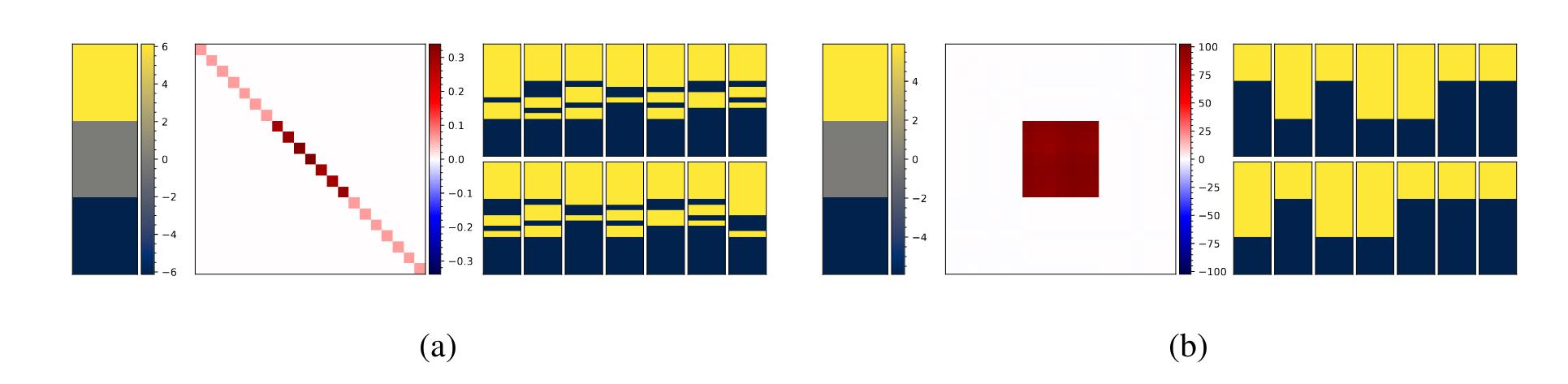
Figure 1 : Results of the toy problem for the diagonal model (a) and a low-rank model (b). From left to rigth : mean, covariance sample and 14 random samples.

What we can see is that both models are able to learn the mean correctly but the diagonal model doesn’t learn the label noise properly. Thus, it generates samples with uncorrelated predictions.

Lund nodule segmentation in 2D

Dataset : LIDC-IDRI dataset 1018 3D thorax CT scans where four radiologists have annotated multiple lung nodules in each scan
Baselines : deterministic U-Net, probabilistic U-Net, PHiSeg model
Metrics : \(DSC\), \(DSC_{nod}\) refers to dice computed only on the slices with nodules.
- \(D_{GED}^{2} = 2\mathbb{E}_{y \sim p, \hat{y} \sim \hat{p}}[d(y, \hat{y})] - \mathbb{E}_{y,y' \sim p}[d(y, y')] - \mathbb{E}_{\hat{y},\hat{y}' \sim \hat{p}}[d(\hat{y}, \hat{y}')]\), where \(d = 1 - IoU(.,.)\) and \(p\) and \(\hat{p}\) are the ground-truth and predictions distributions.
- sample diversity is simply \(\mathbb{E}_{\hat{y},\hat{y}' \sim \hat{p}}[d(\hat{y}, \hat{y}')]\)
Two training configurations :
- Only one of the four set of annotations is used (each set represents a different expert)
- The four sets of annotations are used

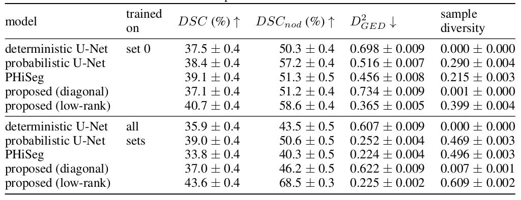
Figure 2 : Quantitative results on the LIDC-IDRI dataset

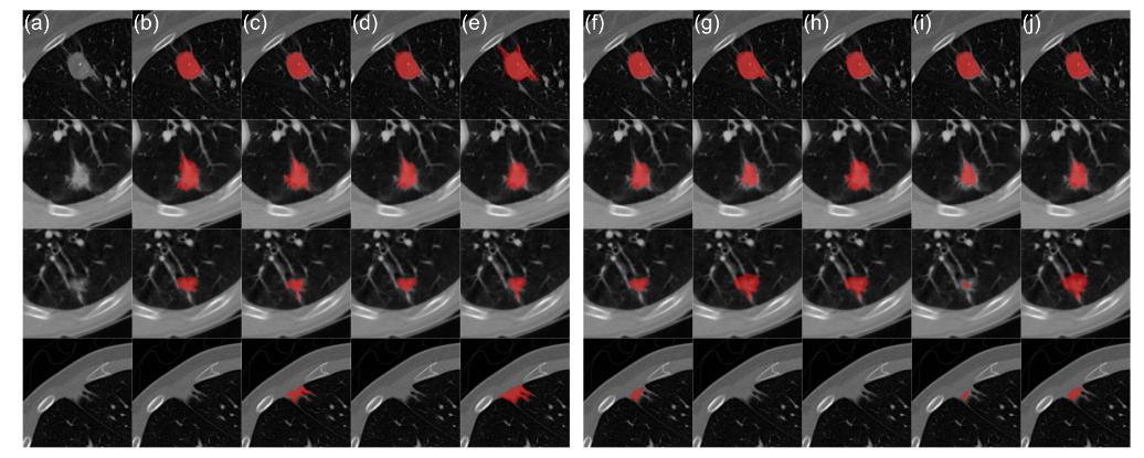
Figure 3 : Qualitative results on the LIDC-IDRI dataset for the proposed model trained on four expert annotations: (a) CT image; (b-e) radiologist segmentations; (f) mean prediction; (g-j) samples

In terms of segmentation, the proposed method (low rank model) outperforms the baseline models in both configurations. It’s also the model that benefits the most from the additional annotations (Figure 2). For uncertainty calibration, the model yielded the lowest \(D_{GED}^{2}\) score. The low rank model also presents a good sample diversity but the diagonal model collapses to a deterministic model, yielding very little sample diversity (Figure 2).

Brain tumor segmentation in 3D

Method is plugged into a DeepMedic architecture
Two models are trained with patches of \(30mm^{3}\) and \(60mm^{3}\), respectively, to evaluate the influence of computing long range dependencies.

Figure 4 : Quantitative results on the BraTS dataset

The quantitative results show that the proposed model has no drop in performance with respect to the deterministic model. Also the increased patch size didn’t bring better calibration or sample diversity (Figure 4).

Figure 5: Qualitative results on the BraTS dataset: (a) T1ce slice; (b) ground-truth segmentation; (c) prediction of deterministic model; (d) prediction of proposed model; (e) marginal entropy; (f-h) samples. Samples were selected to show diversity.

From a qualitative point of view, it is interesting to observe that between different samples an entire region of the segmentation can appear or disappear (Figure 5 row 4), showing the dependencies between the pixels. We can also observe that some samples can correct errors made by the deterministic model (Figure 5 row 2).

Figure 6: Distribution of sample average class DSC per case. The yellow bars denote the fraction of samples whose DSC is higher than the mean prediction, which is represented by a cross. The dashed line is the average fraction of samples better than the mean prediction (average height of the bars).

The distribution of samples DSC per case show that most samples give a DSC worst than the mean prediction (represented by a cross in Figure 6). However, on average, 26% of the samples are better than the mean prediction, showing that we can increase performance by finding the right sample. It is also interesting that the number of samples better than the mean prediction is higher for cases with low performance (difficult cases).

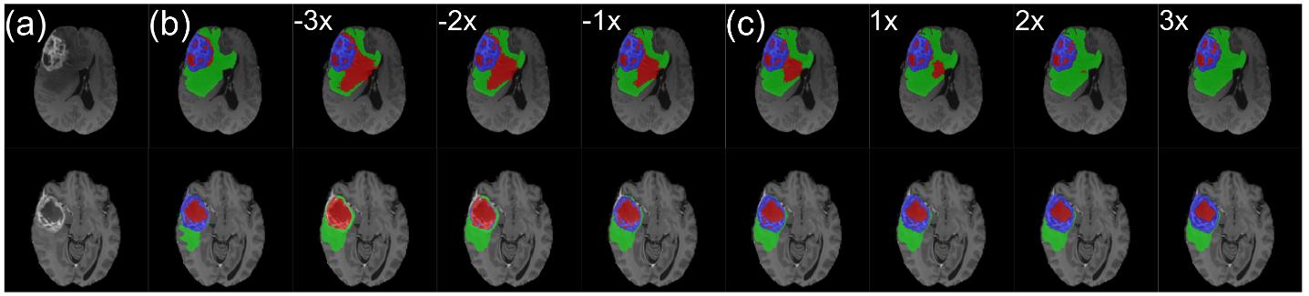
Figure 7: Sample manipulation after inference: (a) T1ce slice; (b) ground-truth segmentation; (c) sample surrounded by manipulated sample with scaling ranging from -3x to 3x.

An other interesting feature is the possibility to manipulate the sample after inference to increase or reduce the presence of a class (Figure 7).

Conclusion

This paper introduces a method for modeling spatially correlated aleatoric uncertainty in segmentation. The method is simpler than previous methods and yields overall better results in segmentation and sample diversity performances. The method is also easy to plug into any architecture, and the ability to generate multiple samples and to manipulate samples is of interest for semi-automatic pipelines.