Revisiting the Calibration of Modern Neural Networks

Highlights

• ViT are well calibrated compared to past models, and are more robust to distribution shift
• When in distribution : calibration slightly deteriorates with model size, but is outweighed by an improvement in accuracy
• Under distribution shift, calibration improves with model size, reversing the in-distribution trend
• Model size and pretraining cannot fully explain calibration differences between model families

Notes

• Quick recap of the key concepts in calibration using Guo et al. paper
• More interesting results with Minderer et al. paper

Introduction

For the introduction of the key concepts, let’s go back to the article of Guo et al., On Calibration of Modern Neural Networks, ICML 2017.

Calibration

A model is well-calibrated if the predicted confidence scores represent a good approximation of the actual probability of correctness.

For example : if we have 100 images predicted cancer with a score of 80%, we expect 20 predictions to be wrong.

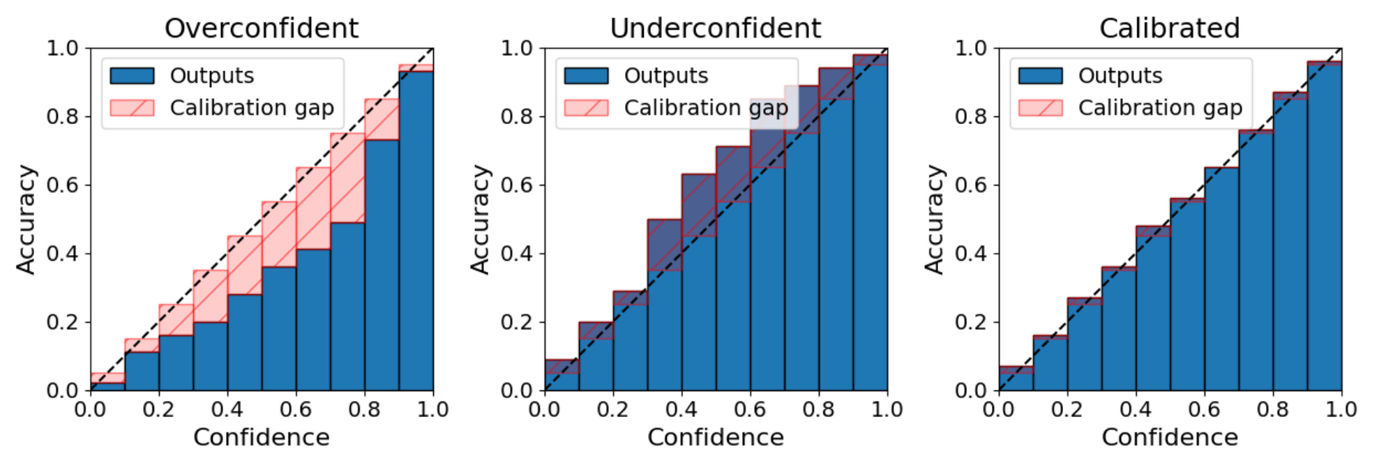
How to measure calibration ? Two simple way, first visually and then quantitatively.

Reliability histogram

Group the predicted scores into bins, and plot the observed accuracy vs the expected accuracy. In more details :

For a set of \(N\) images, we define the true class of the \(i\)-th image \(y_i\) and \(p_i = (p_{i1}, ..., p_{iK})\) the confidences scores of the \(K\) classes. The predicted class \(\hat{y}_i\) is the top-1 classification prediction, that is the class with the greatest confidence score, denoted \(s_i\): \begin{equation} \hat{y}_i = \underset{k \in [1, K]}{\arg\max} : p_i \hspace{0.5cm} \text{and} \hspace{0.5cm} s_i = \underset{k \in [1, K]}{\max} : p_i \end{equation}

For \(M\) evenly spaced bins, we can define \(b_m\) the set of indices \(i\) such as \(s_i \in ]\frac{m-1}{M}, \frac{m}{M}]\) and compute the average bin accuracy and the average bin confidence score :

\begin{equation} \operatorname{acc}\left(b_m\right) = \frac{1}{\left|b_m\right|} \sum_{i \in b_m} \mathbb{1}\left(\hat{y}_i=y_i\right) \end{equation}

\begin{equation} \operatorname{conf}\left(b_m\right) = \frac{1}{\left|b_m\right|} \sum_{i \in b_m} s_i \end{equation}

Expected Calibration Error

ECE is defined as the bin-wise calibration error weighted by the size of the bin :

\begin{equation} \mathrm{ECE}=\sum_{m=1}^M \frac{\left|b_m\right|}{N}\left|\operatorname{acc}\left(b_m\right)-\operatorname{conf}\left(b_m\right)\right| \end{equation}

Temperature Scaling

Temperature scaling is a post-processing method to improve the calibration of the model after the training. The scores predicted by the model are rescaled by a temperature parameter \(T > 0\) using a generalization of the softmax function :

\begin{equation}\label{eq:1} p_{ij} = \frac{\exp^{z_{ij}/T}}{\sum_{k=1}^K \exp^{z_{ik}/T}} \end{equation}

Guo et al. conclusions on the calibration of “modern” networks of 2017 :

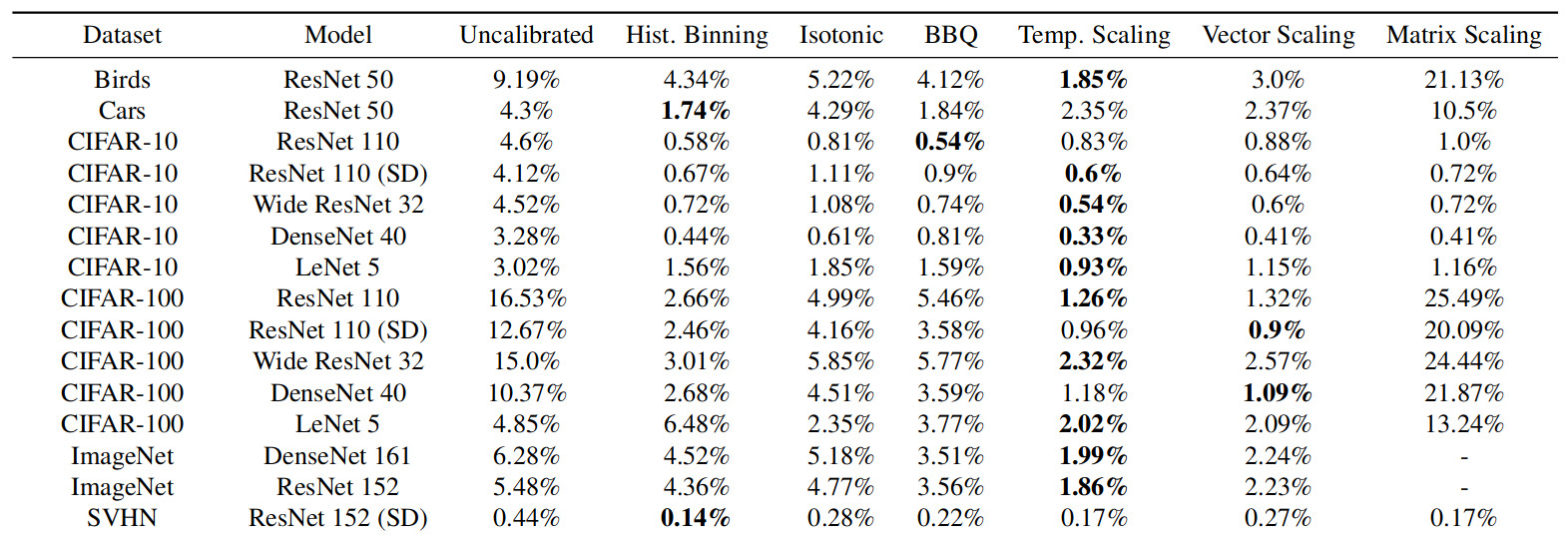
• Deep Learning models are poorly-calibrated : often very overconfident
• Temperature Scaling is very effective to improve the calibration of these models

Why “Revisiting the Calibration of Modern Neural Networks” ?

• Are recent state-of-the-art network still badly calibrated ?
• Do more accurate (and larger) models produce poorly calibrated prediction ? i.e is there a compromise between accuracy and calibration ?
• How does pretraining affect calibration ?

Methodology

Model families

CNN, Transformers, self-supervised and zero-shot models : MLP-Mixer , ViT , BiT , ResNext-WSL , SimCLR , CLIP and AlexNet . With variant of different model size.

All models are trained/finetuned on ImageNet training set, except for CLIP.

Datasets

Different datasets for out-of-distribution benchmarks : ImageNet-V2 (same distribution), ImageNet-C (corruption) , ImageNet-R (art, cartoons, deviantart, graffiti, etc. ) and ImageNet-A (hard samples)

For temperature scaling, they use 20% of the validation set to compute the optimal temperature and report the metrics on the remaining 80%.

In-distribution calibration

Recent model families (ViT, BiT, MLP-Mixer) are both very accurate and well calibrated compared to old models (AlexNet, Guo et al.).

In addition, CLIP is well-calibrated given its accuracy.

Figure 1. ECE vs Error Rate (left) and reliability histogram (right). Marker size indicates relative model size.

Difference between model families still hold after temperature scaling.

Within families, larger models have higher accuracy but also higher calibration error. However, at any given accuracy, ViT models are better calibrated than BiT models. Therefore, model size can not fully explain the intrisic calibration difference between families.

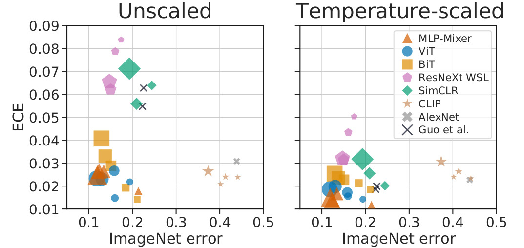
Figure 2. Before and after temperature scaling.

More training date improves the accuracy of the BiT model, but has no significant effect on the calibration.

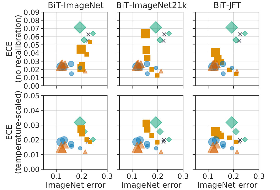
Figure 3. With different pre-training datasets

Conclusion : modern neural networks combine high-accuracy and SOTA calibration, both before and after temperature scaling. Model size and pretraining amount do not fully explain the intrisic difference between the families.

Accuracy and calibration under distribution shift

As expected classification and calibration error increase with distribution shift. The decay in calibration performance is slower for ViT and MLP-Mixer than the other families.

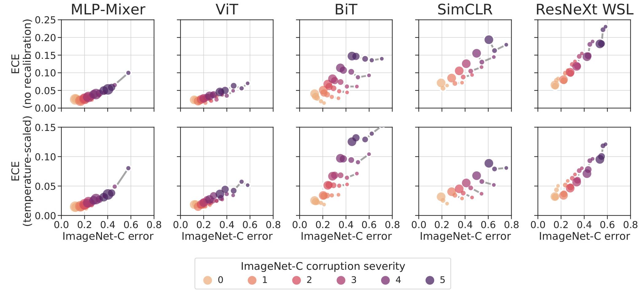
Figure 4. Calibration and accuracy on ImageNet-C.

When in-distribution, we observed that larger models had higher calibration error. But the trend is reversed as we move out of the distribution.

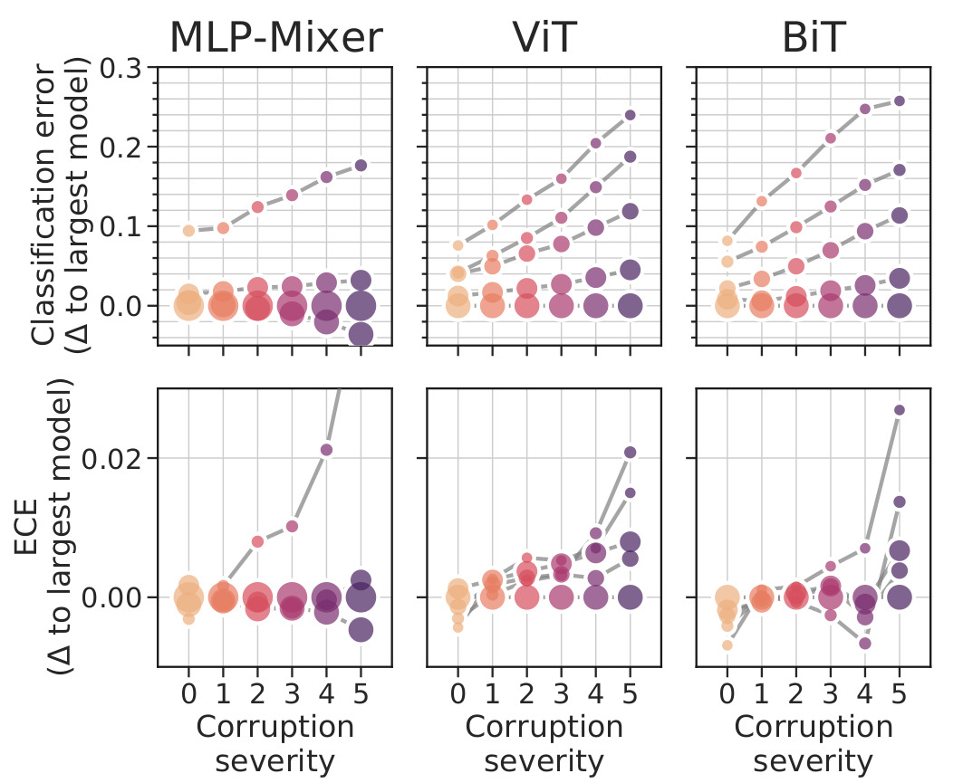
Figure 5. Classification error and ECE for the top three families on ImageNet-C, relative to the largest model variant in each family.

When looking at natural distribution shift (ImageNet-V2, ImageNet-R and ImageNet-A), the ranking between the families is consistent with ranking on ImageNet.

Models that are Pareto-optimal (i.e. no other model is both more accurate and better calibrated) on ImageNet remain Pareto-optimal on the OOD datasets.

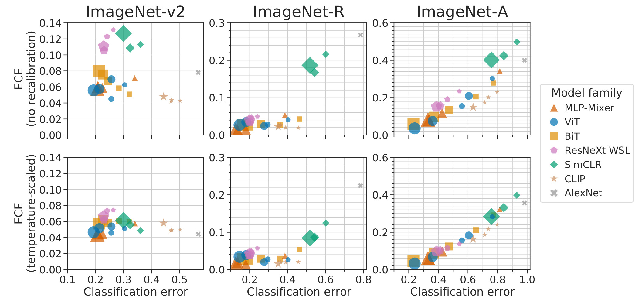
Figure 6. Calibration and accuracy on out-of-distribution benchmarks.

Conclusion :

• The calibration of larger models is more robust to distribution shift.
• Out-of-distribution calibration tends to correlate with in-distribution calibration and out-of-distribution accuracy.