Highlights

The authors propose ImageBind, an approach to learn a joint embedding space across six different modalities.
It is trained in a self-supervised fashion only with image-paired data, but can successfully bind all modalities together.
It is evaluated on many downstream applications, such a zero- and few-shot classification, cross-modal retrieval and generation.

Context and objectives

Many recent works have focused on aligning image features with other modalities, such as text or audio. Such networks, like the popular CLIP¹, exhibit strong zero-shot performances on downstream tasks and provide powerful feature extractors. However, they are limited to pairs of modalities for training and resulting downstream tasks.

The main goal of the authors is to learn a single shared multimodal embedding space by using only image-paired data. In doing so, they place images as anchor modality and suppress the need for building other paired datasets. Moreover, it does not require datasets where all modalities co-occur with each other. ImageBind can successfully link modalities that have not been seen together during training, like audio and text.

ImageBind

Figure 1. Overview of ImageBind.

ImageBind uses pairs of modalities \((\mathcal{I}, \mathcal{M})\) where \(\mathcal{I}\) represents images and \(\mathcal{M}\) another modality. In their work, \(\mathcal{M}\) can be text, audio, depth sensor data, thermal data, and Inertial Measurement Unit (IMU, times-series data from accelerometers and gyroscopes). Note that image can be replaced by video by inflating patch projection layers, thus both are considered as anchor modality and treated with the same encoder.

Each modality \(M\) has its own dedicated encoder (see below for details) and an associated projector \(f_\mathcal{M}\), so that every modality embedding ends up in a space of common dimension.

The model is trained with the standard InfoNCE contrastive loss². Given a batch of observations, it aims to make the embeddings of a pair (\(\mathcal{I}_i\), \(\mathcal{M}_i\)) closer while pulling away the ‘negative’ observations, that is all the other pairs of data in the batch. The loss can be written :

\[\mathcal{L}_{\mathcal{I},\mathcal{M}} = - \log \frac{\exp(\textbf{q}_i^T \textbf{k}_i / \tau)}{\exp(\textbf{q}_i^T \textbf{k}_i / \tau) + \sum_{i\neq j} \exp(\textbf{q}_i^T \textbf{k}_j/\tau)}\]

Modality encoders details

Image and video : Vision Transformer (ViT). For video , they use 2-frame clips, with a video patch of size \(2 \times 16 \times 16\) (\(T\times H \times W\)). Encoder weights are inflated to work with spatiotemporal patches and at inference, features from successive 2-frame clips are aggregated. They leverage image-text supervision from large-scale data by using OpenCLIP’s image encoder weights (ViT-H, 630M parameters). The weights are kept frozen.
Audio : Audio samples are recorded at 16kHz. They are cut into 2-second samples and converted into spectrograms using 128-mel spectrograms bins. Spectrograms are processed as images with ViT with a patch size of 16 and stride 10.
Text : They directly use CLIP’s encoder architecture, which is a VIT. Again, they leverage image-text supervision from large-scale data by using OpenCLIP’s text encoder weights (320M parameters). The weights are kept frozen.
Depth and Thermal data : They treat both as one-channel images and use ViT to encoder them.
IMU : The 6-channel signal acquisition is cut into 5-second clips, giving 2K time steps IMU. They are projected using 1D convolution with kernel size of 8 and then encoded using a Transformer.

Experiments

Datasets

The authors use several datasets to couple audio, depth maps, thermal data and IMU to image (or video). For training, they use (video, audio) pairs from Audioset dataset (2M samples), (image, depth) pairs from SUN RGB-D dataset (5K samples), (image, thermal) pairs from LLVIP dataset (12K samples) and (video, IMU) pairs from Ego4D dataset (7K5 samples). They are used together during training, and imbalance between datasets is handled by replicating 50 times SUN RGB-D and LLVIP. These datasets have a test subset for zero-shot evaluation and all other databases in Figure 2 are used for evaluation only.

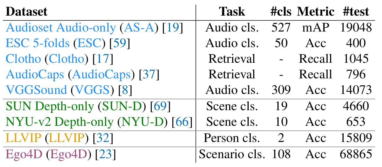
Figure 2. Overview of datasets used.

Emergent zero-shot classification

Zero-shot classification refers to the task of classifying samples for unknown classes or for models that have not been trained specifically on a classification task. It is applicable to models that have been trained to build a common space between paired modalities (\(\mathcal{T}\),\(\mathcal{X}\)), where \(\mathcal{T}\) is text and \(\mathcal{X}\) can be any other modality, such as image or audio. For such models, it is possible to perform classification without the need for finetuning specific for this task. The class is determined using simple standard prompts, such as “An image of a {class}”, where {class} is replaced by every possible class. The class attributed to a sample is the one for which the associated text prompt has the highest similarity with the sample.

Here, ImageBind is able to perform zero-shot classification between text and a modality \(\mathcal{M}\) which has not been paired with text during training (audio, depth, etc.). This is an indirect phenomenon that appears thanks to the training with pairs of (image, text) and (image, \(\mathcal{M}\)). Such downstream performances are referred to emergent zero-shot classification by the authors.

Figure 3 shows emergent zero-shot classification performance of ImageBind on all modalities. It is compared to absolute SOTA performances (usually using supervision and ensemble models) and, when possible, to the best text-paired approach. Note that text-image and text-video zero-shot metrics are high because ImageBind’s image encoder uses frozen OpenCLIP’s weights.

Figure 3. Emergent zero-shot classification performances for every modality. Top-1 accuracy is always reported, except for MSR-VTT (Recall@1) and Audioset AS-A (mAP).

Zero-shot retrieval

Even without having been trained with (text, audio) pairs, ImageBind achieves performance that are on par with AudioCLIP, which uses text-audio supervision, and close to supervised baselines. Figure 5 shows that adding audio to video for text-based retrieval (36.8 R@1 against 36.1 on Figure 3)

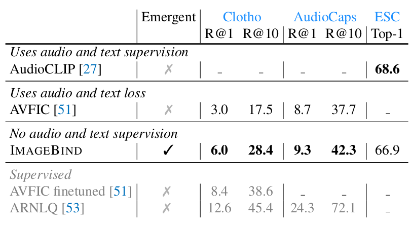
Figure 4. Emergent zero-shot audio-retrival and classification.

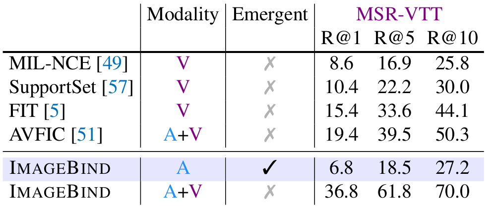
Figure 5. Zero-shot text-based retrieval.

Few-shot classification

On few shot classification, ImageBind’s audio feature extractor is largely superior to AudioMAE (self-supervised reconstruction-based pretraining) and reaches performance on par with supervised models. It also compares favorably to state-of-the-art multimodal SSL pretraining techniques, such as a MultiMAE model trained with images, depth and semantic segmentation masks.

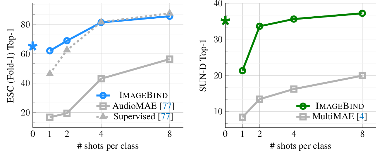
Figure 6. Few-shot performance on audio and depth maps.

Multimodal embedding space manipulation

ImageBind’s joint multimodal embedding space allow for many cross-modal manipulations, such as audio-based generation, modality combination for image retrieval (Figure 7) or object detection with audio queries (Figure 8)³.

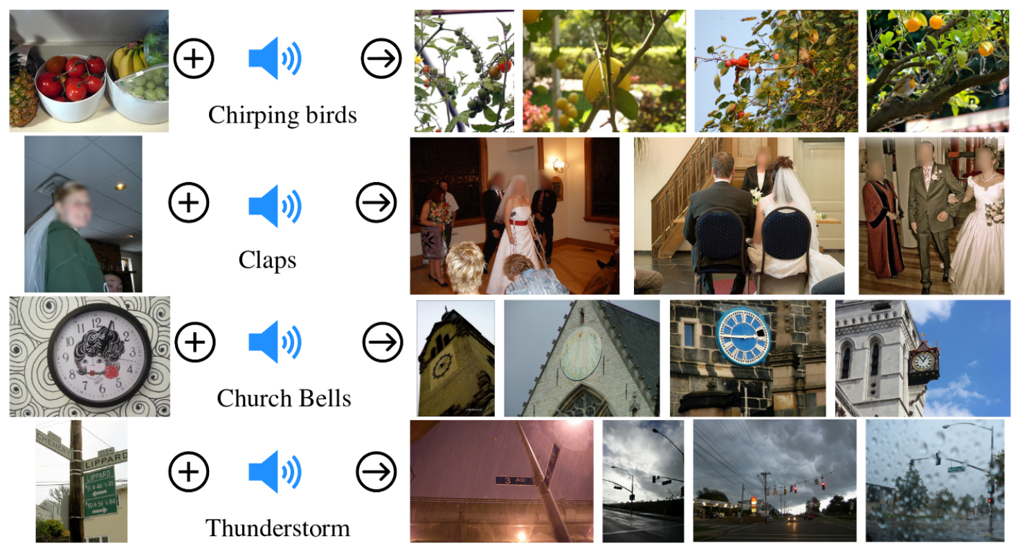
Figure 7. By adding image and audio embedding and using the resulting composed embedding for image retrieval, it capture semantics from the two modalities.

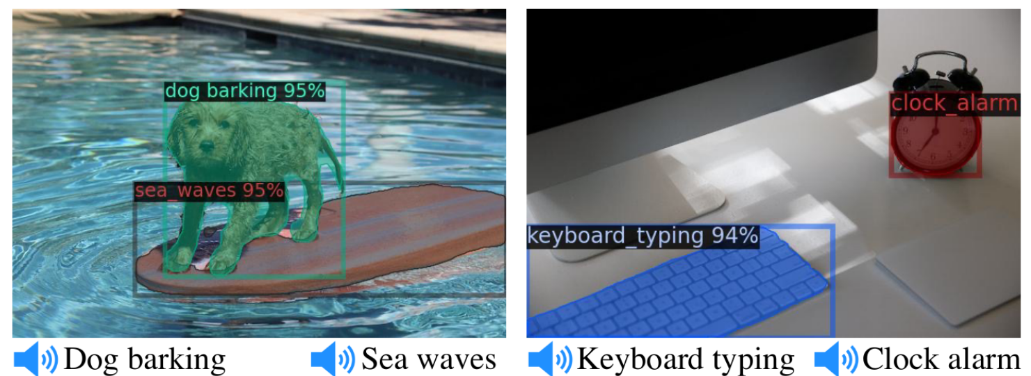
Figure 8. Simply replacing Detic’s CLIP-based ‘class’ embeddings with ImageBind's audio embeddings leads to an object detector promptable with audio, without no additional training required.

Conclusion

ImageBind is an interesting and promising work for all these reasons.

Reference

A. Radford, J. W. Kim, C. Hallacy, A. Ramesh, G. Goh, S. Agarwal, G. Sastry, A. Askell, P. Mishkin, J. Clark, G. Krueger, I. Sutskever, Learning Transferable Visual Models From Natural Language Supervision, International Conference on Machine Learning (PMLR), 2021, lien ↩
A. van den Oord, Y. Li, O. Vinyals. Representation learning with contrastive predictive coding, NeurIPS, 2018, lien ↩
X. Zhou, R. Girdhar, A. Joulin, PP. Krähenbühl, I. Misra, Detecting Twenty-thousand Classes using Image-level Supervision, European Conference on Computer Vision (ECCV), 2022, lien ↩