RePaint: Inpainting using Denoising Diffusion Probabilistic Models
Notes
- Paper’s code is available at this GitHub repo
- A re-implementation of the algorithm is available at the following Monai prototyping repo
- An introduction tutorial about denoising diffusion probabilistic models is available Here
Highlights
- Image inpainting done thanks to Denoising Diffusion Probabilistic Model (DDPM)
- Free-form inpainting, i.e., works with a wide variety of masks
- Inpainting is done during the inference stage, by modifying the generation process, thus not requiring specific training
- The Repaint method outperforms state-of-the-art autoregressive and GAN approaches for at least five out of the six mask distributions tested
Introduction
The task of inpainting is what we define as the process of filling damaged, missing, or hidden areas of an image with meaningful information.
The state-of-the-art of inpainting methods were autoregressive-based or GAN-based approaches, which mostly use a distribution of arbitrary masks to train their models. Resulting in poor generalization capabilities.
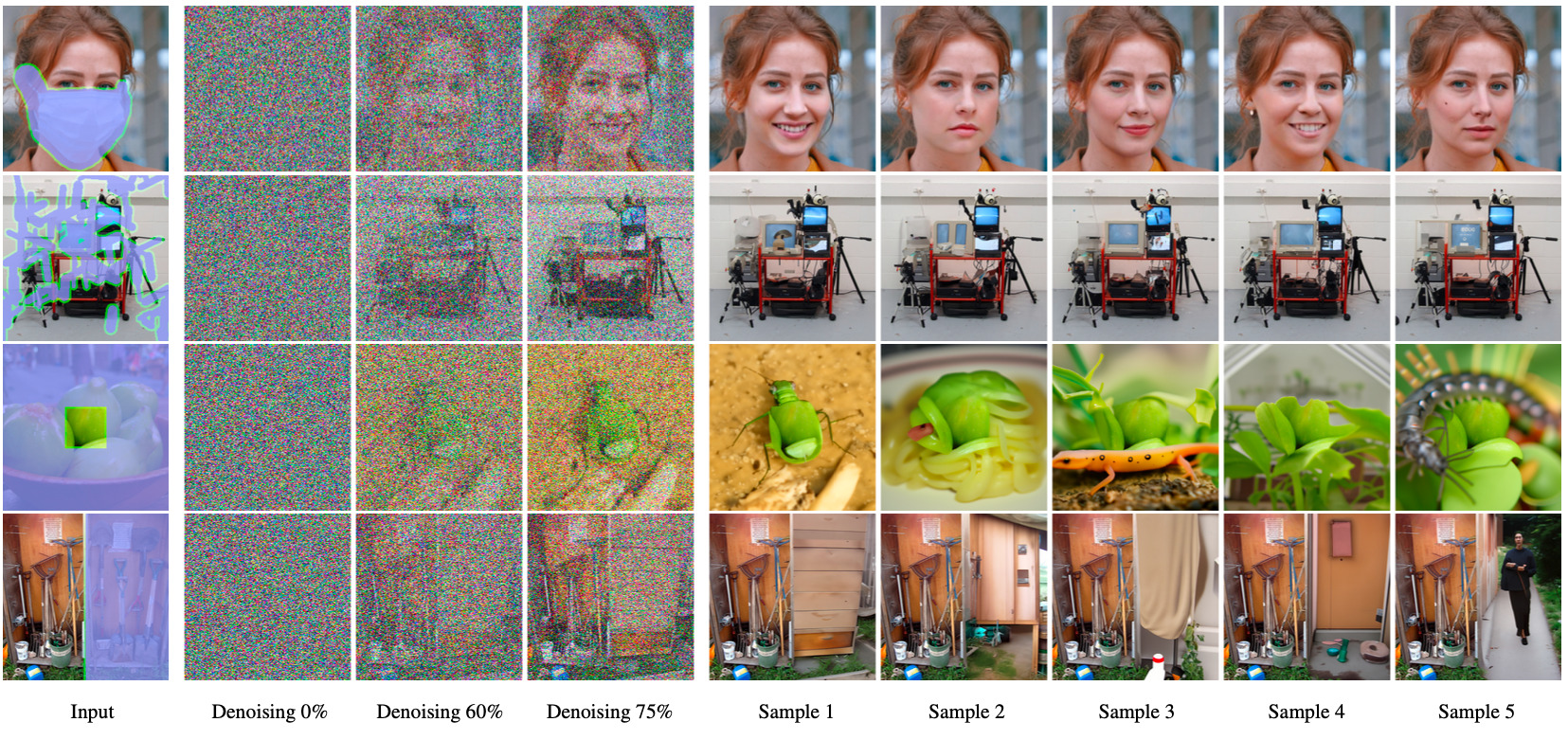
The paper proposes a new method to condition the generation process and was one of the first methods at the time to use diffusion models. This method, the Repaint method, only takes place during the complete generation process of DDPM and does not require specific training of the model.
Prerequisites
A quick reminder about diffusion models is needed to understand the following parts of this post.
Diffusion models are basically networks which through training, try to predict the noise added to an image. We define a range of noise levels from \(0\) to \(T\), \(x_0\) denoting a noise-free image and \(x_T\) denoting a pure Gaussian noise \(\sim \mathcal{N}(0, I)\).
The process of gradually adding noise to an image is called the forward diffusion process, and the action of gradually removing it is called the reverse diffusion process.
The forward diffusion process is modeled as a Markov chain where noise is added gradually at each step, and the prediction of \(x_t\) only depends on \(x_ {t-1}\).
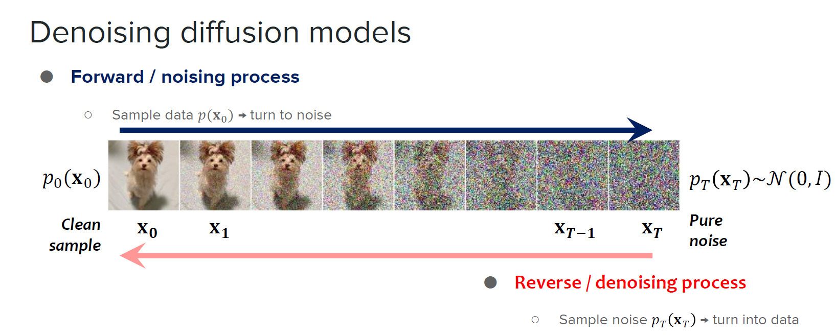
Source : scholar.harvard.edu
Method
Inpainting algorithm and general idea
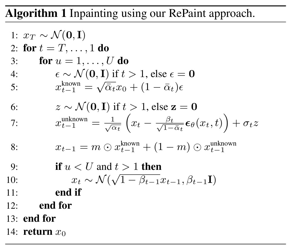
The innovation of the Repaint paper is due to its method of generation, which is conditioned by the known region of the image. They introduce some notations: the ground truth image is denoted as \(x\) and the mask corresponding to the unknown area to inpaint as \(m\). They define their new reverse diffusion process as follows:
\[\begin{aligned} \color{red}{x^{known}_{t−1}} & ∼ \mathcal{N} (\sqrt{\bar{\alpha_t}}x_0, (1 − \bar{\alpha_t})I)\\ \color{green}{x^{unknown}_{t−1}} & ∼ \mathcal{N} (\mu_\theta(x_t, t), \Sigma_\theta(x_t, t))\\ \color{blue}{x_{t−1}} & = m \odot \color{red}{x^{known}_{t−1}} + (1 − m) \odot \color{green}{x^{unknown}_{t−1}} \end{aligned}\]
The inpainting process explained in the paper is rather simple. If we want to generate \(x_{t-1}\) output from \(x_t\) input we have to :
- generate through forward diffusion from \(x_0\) a noisy image at \(t-1\) noise level
- generate the \(x_{t-1}\) image from \(x_t\) using reverse diffusion
- concatenate the known part of the forward diffusion with the unknown part of the reverse diffusion
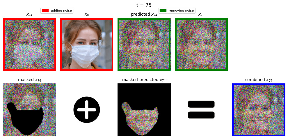
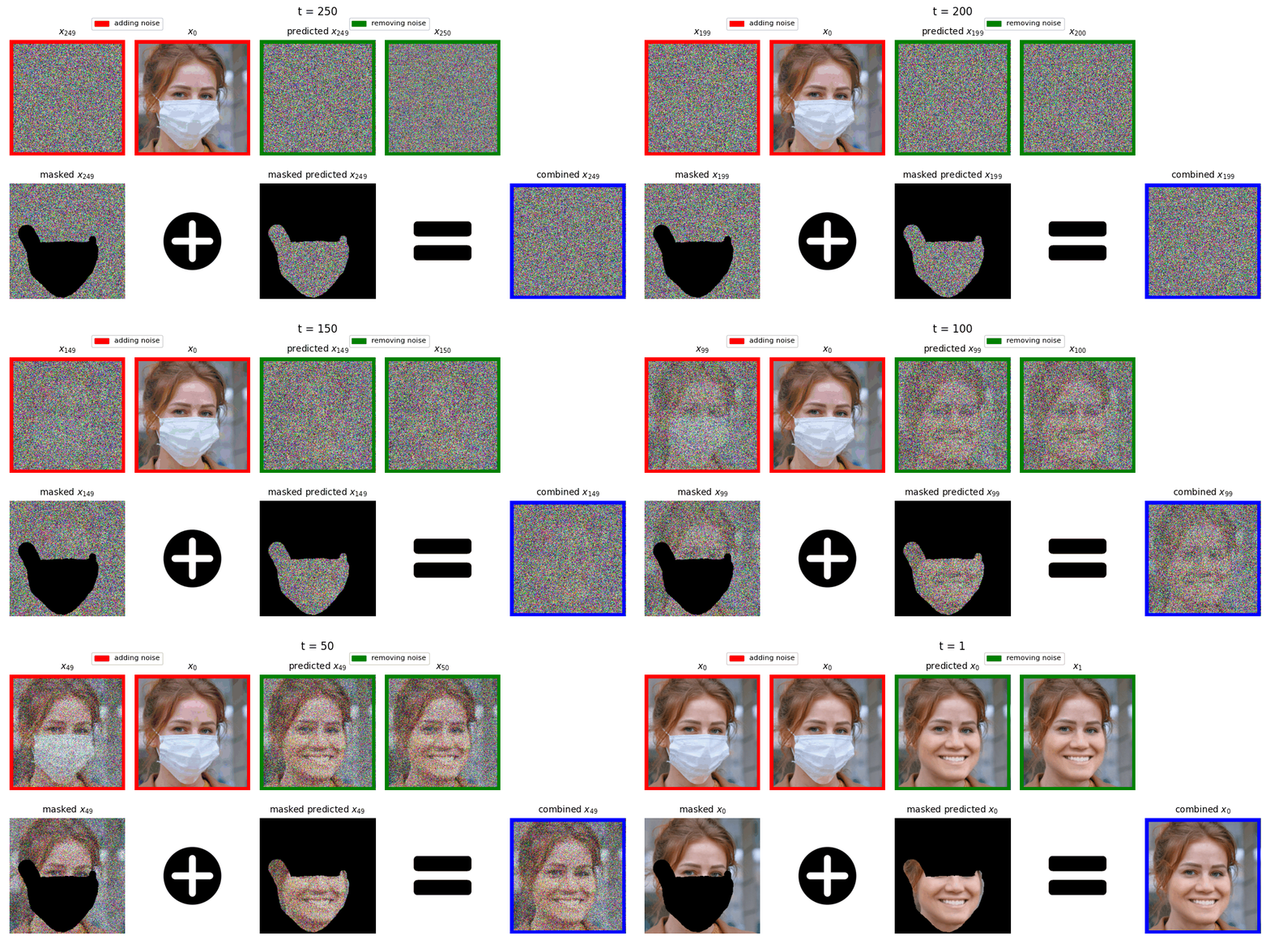
Basically, the idea boils down to sampling from known and unknown regions at a given timestep. Since this sampling is done through all steps of the reverse diffusion process, the distribution of the intermediary images match more and more the properties of the known image at each denoising steps. At the end of the process, the generated image is an image with intact known region, and a texture related to the known region which covers the unknown region.
Resampling
As you may have noticed, the previously described reverse diffusion process does not directly restrict diffusion process generation. This can result in a coherent generated texture by itself, but incoherent regarding the general image semantic, with non-matching boundaries, for instance (cf. figure 3, with n from 1 to 5).
To overcome this problem, the authors leverage the fact that DDPM is trained to create images that lie within a data distribution and diffuse the output \(x_{t−1}\) back to \(x_t\). The effect of this is to incorporate some information in the \(x^{unknown}_t\) and add noise to the image. In consequence, the model gain in accuracy to approximate the distribution that correspond to the image the user is trying to inpaint, thus creating new \(x^{known}_t\) and \(x^{unknown}_t\) regions that are better harmonized.

As you can see, the more resamples are made, the better harmonized the resulting image is. The authors noted that after about 10 resamplings, the benefits of resampling are negligible (it still adds noise to the image, so it’s not completely useless). Adding those resampling steps makes the inferring process look like this:
Results
Metrics
To put into perspective their results, the authors compared their method to others, which are autoregressive-based or GAN-based approaches. All the methods were trained on two datasets: CelebA-HQ and ImageNet. The comparisons are done using the perceptual metric LPISP, learned on the deep feature space of AlexNet, and a user study.
The user study is done by showing each voter the reference image to inpaint and two inpainted images, one using Repaint and the other using another method. The five people who had participated in the voting had to vote for the most realistic inpainting, resulting in 1000 votes per method-to-method comparison in each dataset and mask setting (Wide, Narrow, Every Second Line, Half Image, Expand, and Super-Resolve). The vote distribution shows a 95% confidence interval toward the mean vote.
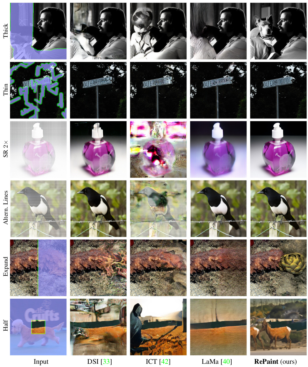

As we can see, the Repaint inpainting method was most of the time chosen by voters as the most fitting inpainting method and has a correct LPIPS regarding the other methods.
Ablation Study
A huge con of the Repaint method is its computational cost. The diffusion model inference process is not fast in the first place, but if you need \(T\) denoising steps to denoise an image, with Repaint you will need \(T \times r\) steps to inpaint an image.
To overcome that problem, the researchers made an ablatation study, doing a trade-off between the number of resampling and the number of denoising steps for a given number of steps.

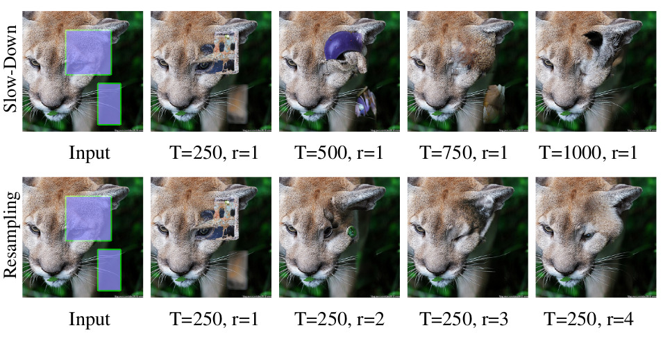
Through that study, they show that for the same computational budget, it is better to increase the number of resamplings to the detriment of the number of denoising steps.
Conclusions
- The proposed inpainting method was the first one using DDPM at the time.
- The quality of the images inpainted is correct, and the method challenges state-of-the-art in this domain.
- Other promising methods have been developed since Repaint (see also the Copaint method)
- The inpainting is correct regarding the fact training a diffusion model is basically training a U-net to predict noise, instead of training a GAN.