Ultrasound image quality

During ultrasound acquisitions, phenomena such as aberration and reverberation produce unwanted echoes that degrade the image quality. In particular, haze is an artifact that occurs due to multipath reflections and produces a white haze on the echo image.

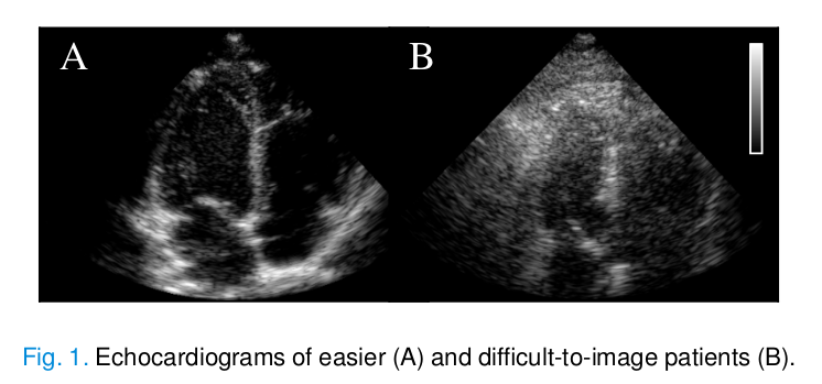
This phenomenon can make diagnosis much more difficult, both qualitative and quantitative.

Existing dehazing techniques:

Harmonic imaging receives echoes at frequencies that are multiples of the original frequency. It produces higher quality images, as multipath scatterers have less energy and therefore generate fewer harmonics. However, it results in reduced penetration depth.
Clutter filtering methods.
- Block-matching and 3D filtering algorithm (BM3D) works by grouping similar patches of the image and then stacking and filtering them. It needs assumptions on the noise distribution.
- Temporal decompositions (PCA, SVD) allow to separate data correspoding to rapidly moving events (tissue) from data corresponding to stationary events (clutter). This assumption is not always true, leading to mistakes.
- etc.
Deep learning methods. Supervised approaches have been implemented to supress reverberation haze. They require of a supervised dataset and may have difficulty to generalize across datasets.

The authors propose to perform dehazing as a post-processing step with diffusion models, which can model highly complex data distributions without having to rely on basic assumptions. In particular, they model the distribution of both clean tissue and haze using two separate score-based networks. Then, they perform posterior sampling for dehazing.

Methods

Formulation of the dehazing process

Backscattered echoes are received by the ultrasound probe. The resulting ultrasound signal \(y\) consists of the sum of received echoes from the tissue \(x\) and all multipath haze echoes \(h\) :

\[y = x + h.\]

The dehazing problem can be written as a source separation task, where the dehazed signal \(x\) has to be retrieved from the acquired signal \(y\) . This is an ill-posed inverse problem.

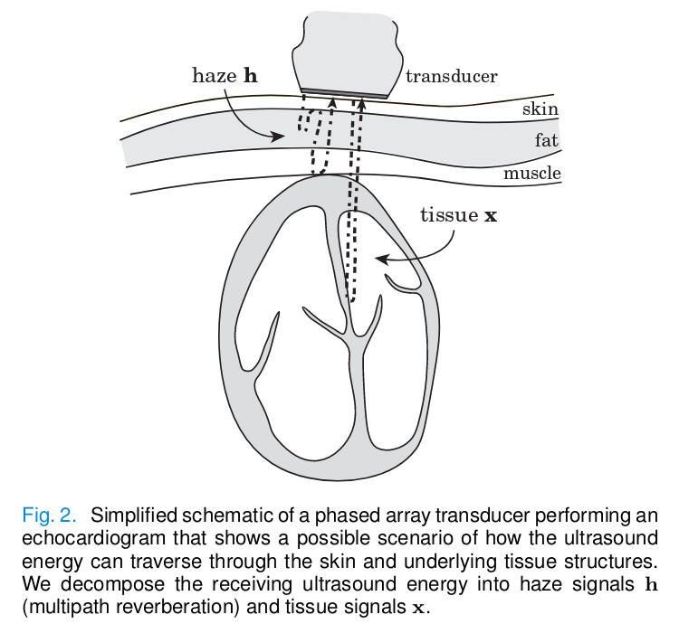
From a probabilistic point of view, sampling from the posterior distribution \(p_{X,H}(x,h|y)\) we can find the optimal \(\hat{x}\) and \(\hat{h}\) given the measurement \(y\) and prior knowledge. Using Bayes’ rule, the posterior can be written as:

\[(x,h) \sim p_{X,H}(x,h|y) \propto p_{Y|X,H}(y|x,h) \cdot p_X(x) \cdot p_H(h),\]

where \(p_{Y|X,H}(y|x,h)\) is the likelihood and \(p_X(x)\) and \(p_H(h)\) are prior distributions of tissue and haze. This formulation allows us to model the haze distribution as any arbitrarily complex distribution and not only Gaussian, as haze is known to be structured and spatially correlated. Tissue and haze prior distributions are learned using score-based models.

Score-based diffusion models

The main idea of score-based models is to represent a probability distribution \(p(x)\) by modeling the gradient of the log probability density function \(\nabla_x \log{p(x)},\) known as the score function.

In a diffusion process, clean data \(x\) from distribution \(p(x)\) is corrupted to some distribution \(\pi(x)\) through a sequence of Gaussian perturbations. It can be written in a simplified form using the following stochastic differential equation (SDE):

\[dx_t = \sigma^t dw,\]

where \(\sigma\) accounts for the diffusion trajectory at time step \(t,\) \(w\) denotes Brownian motion and \(dw\) infinitesimal white noise.

We want to reverse the diffusion process so that we can sample from \(p(x).\) The reversed process can be written as a reverse-time SDE:

\[dx_t = -\sigma^{2t} \underbrace{\nabla_{x_t} \log p(x_t)}_\text{score}dt + \sigma^t dw_t,\]

where the score function needs to be estimated. It can be learned by a neural network \(s_{\theta}(x_t,t)\) that can be optimized using the denoising score-matching method (DSM) with the following objective:

\[\theta^* = \underset{\theta}{\operatorname{arg min}} E_{t \sim U[0,1]} \bigl\{ E_{x \sim p(x), x_t \sim q(x_t|x)} [ ||s_{\theta}(x_t,t) - \nabla_{x_t} \log q(x_t|x)||_2^2 ] \bigr\},\]

where \(q(x_t|x_0) \sim N(x_0, \sigma^t)\) is the perturbation kernel of the diffusion process. With a sufficiently large dataset, DSM enables approximating the true score \(s_{\theta}(x_t,t) \simeq \nabla_{x_t} \log p(x_t).\)

Then, during inference the learned score function is substituted in the reverse-time SDE and the reverse-time diffusion process is discretized in a series of time steps and solved with the Euler-Maruyama method. The update rule is given by:

\[x_{t-\Delta t} = x_t - \sigma^{2t} s_{\theta}(x_t)\Delta t +\sigma^t \sqrt{|\Delta t|}z,\]

where \(z \sim N(0,1).\) The score-based denoising term moves the solution towards \(p(x)\) and the second term corrupts it again to correct errors made in earlier sampling steps to prevent solutions to converge solely to high-density regions.

(For more details, look at the tutorial on score-based diffusion models.)

Proposed dehazing method

The authors tailored several techniques used in deep learning and diffusion models to efficiently apply them to ultrasound data.

Joint posterior sampling

The idea is to combine two prior distributions during posterior sampling by sampling from them in parallel whilst conditioning on the measurement.

The joint posterior sampling \(p_{X|Y}(x,h|y)\) is achieved through the formulation of a joint conditional diffusion process \(\{x_t,h_t|y\}_{t \in [0,1]},\) that gives a joint conditional reverse-time SDE:

\[d(x_t,h_t) = - \sigma^{2t} \nabla_{x_t, h_t} \log p(x_t,h_t|y)dt + \sigma^t dw_t.\]

From the Bayesian formulation presented at the beginning, we can construct two separate diffusion processes defined by two different score models: \(s_{\theta}(x_t,t) \simeq \nabla_{x_t} \log p(x_t)\) and \(s_{\psi}(h_t,t) \simeq \nabla_{h_t} \log p(h_t).\) The gradients of the posterior with respect to \(x\) and \(h\) are:

\[\begin{equation*} \begin{cases} \nabla_{x_t} \log p(x_t,h_t|y) \approx s^*_{\theta}(x_t,t) + \nabla_{x_t} \log p(y|x_t,h_t) \\ \nabla_{h_t} \log p(x_t,h_t|y) \approx s^*_{\psi}(h_t,t) + \nabla_{h_t} \log p(y|x_t,h_t) \end{cases} \end{equation*}\]

Then, substituting the posterior in the joint conditional reverse-time SDE allows to sample from the posterior and eventually obtain both the dehazed signal \(x\) and the haze estimation \(h.\)

Finally, the likelihood \(p(y|x_t,h_t)\) is usually intractable and has to be approximated. A solution is to corrupt the measurement \(y\) along the diffusion process \(\{y_t\}_{t\in[0,1]}.\) We obtain the projected value \(\hat{y}_t \sim q(y_t|y_0),\) which is an approximation of the noise-perturbed likelihood:

\[p(y|x_t,h_t) \approx p(\hat{y}_t|x_t,h_t) \sim N(x_t + h_t, \rho^2I).\]

Learning ultrasound priors

Usually, generative models are used for applications in the image domain. In the case of ultrasound signals, some considerations need to be taken into account.

In particular, ultrasound data has a high dynamic range compared to images that make activation functions to work suboptimally and can slow down the training process.

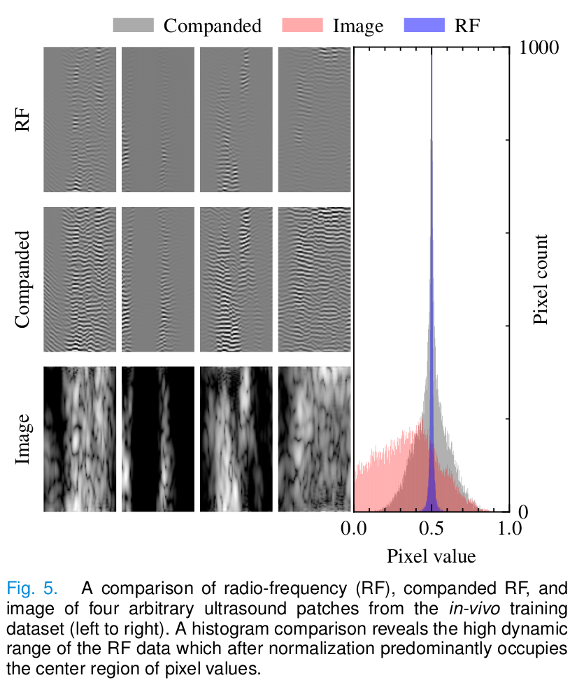
As a solution, companding is used to compress and expand the dynamic range of a signal.

\[C(x_{RF}) = \text{sgn}(x_{RF})\frac{\ln(1+\mu|x_{RF}|)}{\ln(1+\mu)}, \hspace{1cm} -1 \leq x_{RF} \leq 1,\] \[C^{-1}(x) = \text{sgn}(x)\frac{(1+\mu^{|x|}-1)}{\mu}, \hspace{1cm} -1 \leq x \leq 1.\]

During compression, the signal is transformed to the logarithmic domain and its dynamic range is reduced. As a result, the companded data has a distribution that is more similar to the image pixel distribution.

However, a consistency step is needed during the diffusion process to be coherent with the two different domains:

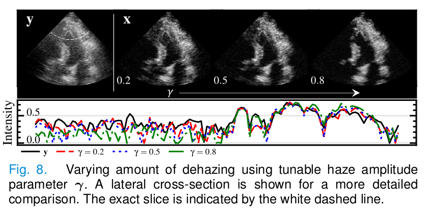
\[\nabla_{x_t} \log{p(y|x_t,h_t)} \approx \nabla_{x_t} \log{p(\hat{y}_t|x_t,h_t)} = ...\] \[\lambda \nabla_{x_t} ||\hat{y}_t - C(x_{RF,t}+h_{RF,t})||_2^2 = \lambda \nabla_{x_t} ||\hat{y}_t - C(C^{-1}(x_t) + \gamma C^{-1}(h_t))||_2^2,\]

where \(\lambda\) is a weighting term for the trade-off between the measurement error and the prior and \(\gamma\) controls the desired signal-to-haze ratio.

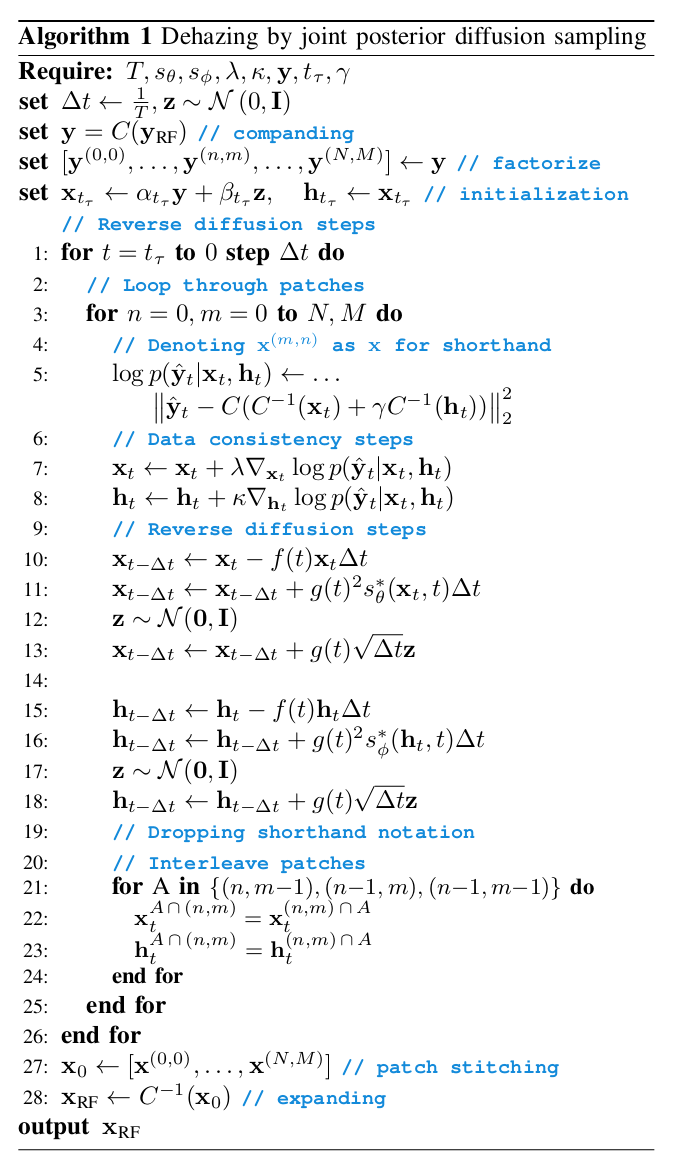
Then, the dehazing procedure by joint posterior sampling works as follows:

Patch-based inference

The patch-based inference has been shown to mitigate overfitting and improve generalization. A method to enforce coherence between reconstructed patches is the mask-shift trick.

The idea is to define \(N \times M\) overlapping patches of the measurement \(y\) to obtain \([y^{(0,0)}, ..., y^{(N,M)}].\) First, one diffusion step is performed on all patches independently, resulting in \([x_t^{(0,0)}, ..., x_t^{(N,M)}].\) Then, the diffusion process of neighboring patches is interleaved and, at each time step, they replace all overlapping pixels of the adjacent patches with the current patch:

\[x_t^{(n,m-1)\cap(n,m)} = x_t^{(n,m)\cap(n,m-1)}\]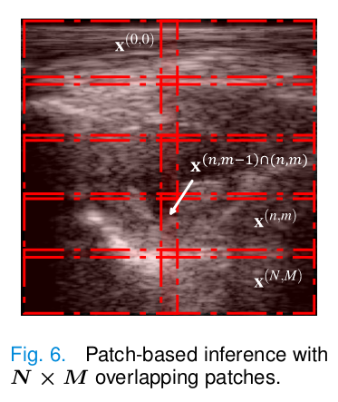

Haze estimation

At train time, a series of haze signals are needed to learn \(s_{\psi}.\) These signals do not have to be paired to tissue measurements. Two ways can be considered to obtain haze signals:

Use a haze phantom in a water tank that simulates multipath reflections.
Consider noisy in vivo ultrasound measurements and extract side lobes and clutter from regions with low SNR.

At inference time, no assumption on haze is needed as the learned haze prior is used.

Initialization

The method come closer diffuse faster (CCDF) is an accelerated sampling scheme that starts the reverse diffusion at \(t_{\tau}\) where \(t_0 \leq t_{\tau} \leq t_T\) instead of starting at \(t_T.\) This simultaneously reduces the number of diffusion steps and also provides a better initial estimate derived from the measurement through a forward diffusion step:

\[x_{t_{\tau}} = \alpha_{t_{\tau}}y + \beta_{t_{\tau}}z.\]

Both tissue signal \(x_{t_{\tau}}\) and haze signal \(h_{t_{\tau}}\) initial estimates are initialized with this method. \(\tau\) is chosen such that there is no significtaive loss in recontruction quality compared with a Gaussian initialization.

Training and inference details

Training:
- Architecture for the tissue and haze score models: NCSNv2 (similar to U-Net).
- Patch size of \(128 \times 64.\)
- 100 epochs, batch size 8, learning rate 1e-4.
- Augmentation through random left-right flips and random brightness offset uniformly sampled in [-0.1, 0.1].
Inference:
- The diffusion trajectory is controlled by \(\sigma = 25.\)
- The initialization is defined by \(\alpha_{t_\tau} = 1\) and \(\beta_{t_\tau} = \frac{\sigma^{2t}-1}{2\log{\sigma}}.\)
- Diffusion is ran for \(T=200\) steps and starts at \(\tau = 160.\)
- Parameters \(\lambda \approx 0.5\) and \(\kappa \approx 0.5.\)
- 10% overlap between adjacent patches to interleave the diffusion process.

The dehazing is performed as follows:

Experiments

In vitro

Acquisition of 150 frames from a heart phantom to train the \(s_\theta\) tissue model and 38 frames for validation.
Acquisition of 150 frames from a haze phantom to train the \(s_\psi\) haze model and 38 frames for validation.
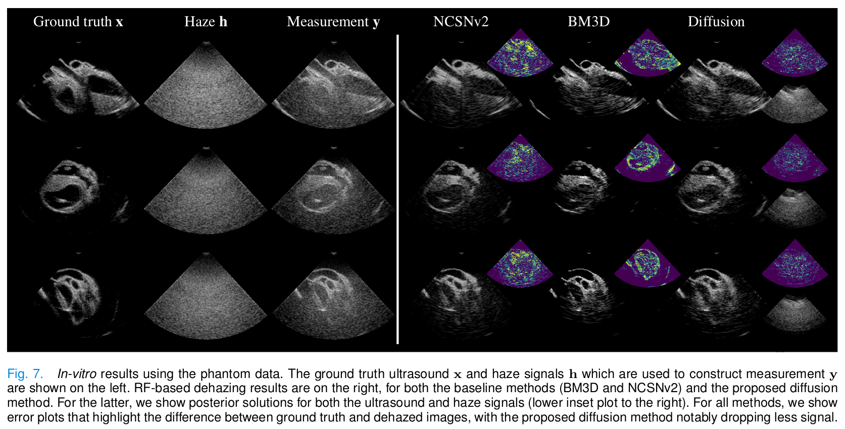
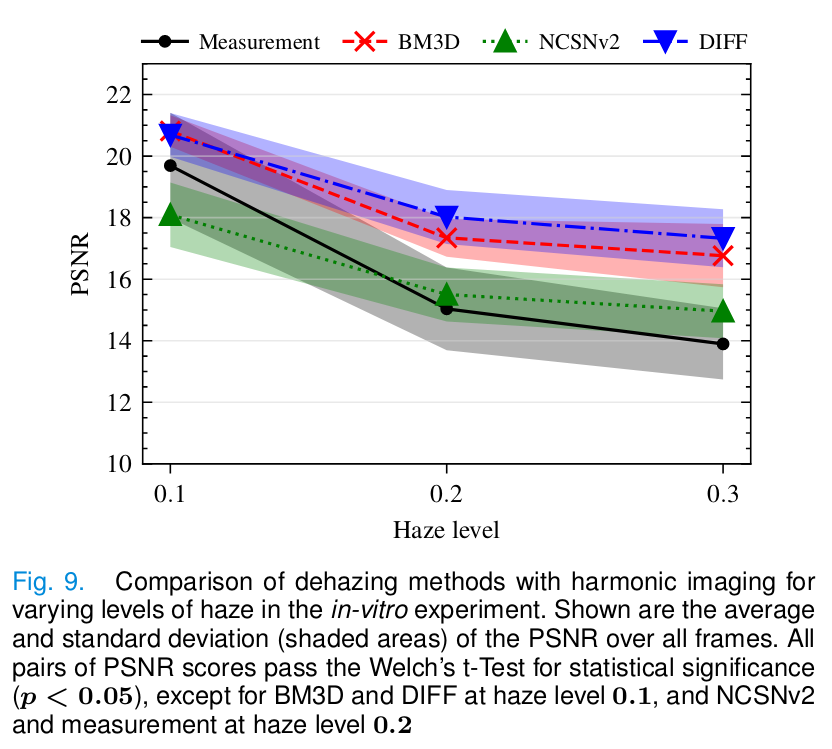
During inference, the haze signals were added to the heart phantom with varying haze levels. This allowed to have ground truths.

In vivo

1500 “clean” frames from three volunteers used to train the tissue model.
120 frames from one difficult-to-image volunteer used to train the haze model.
1020 frames from two difficult-to-image volunteers for validation.

Baselines

BM3D adapted and fine-tuned for the cardiac dehazing problem.
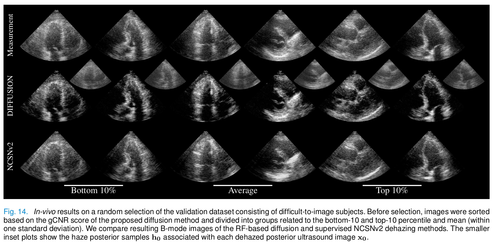
Supervised deep learning approach based on NCSNv2 (U-Net) trained on the supervised phantom dataset.

Metrics and downstream delineation task

For the in vitro experiment: peak signal-tonoise ratio (PSNR).
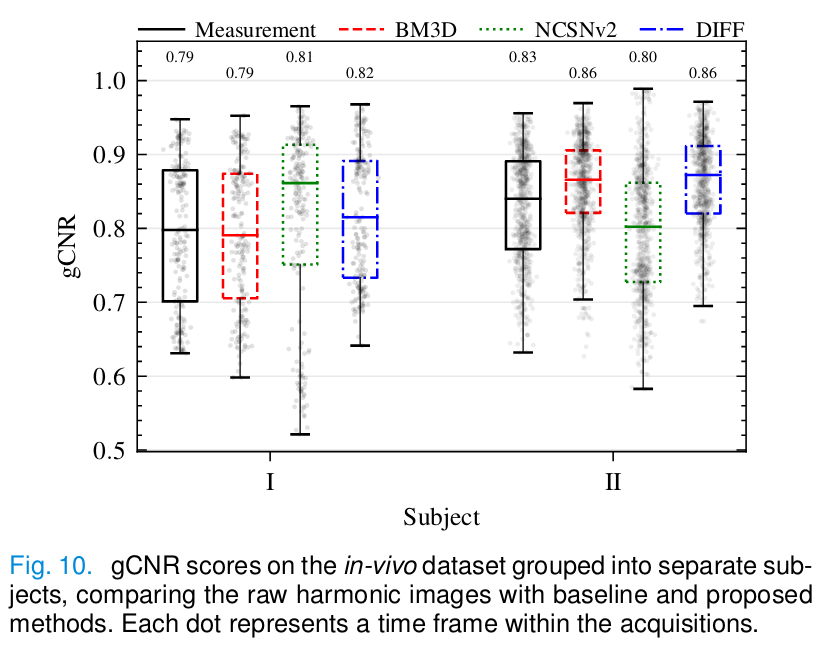
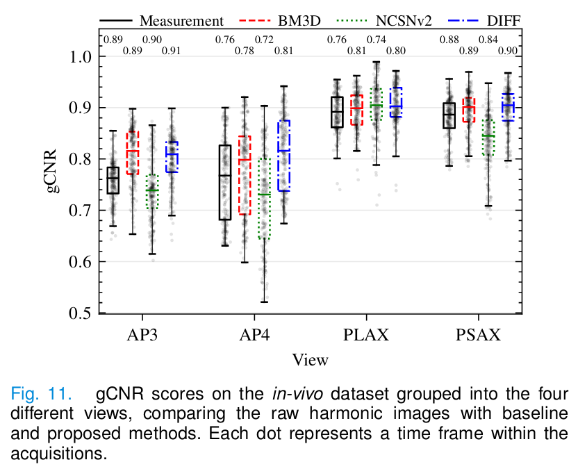
For the in vivo experiment: generalized contrast-to-noise ratio (gCNR).
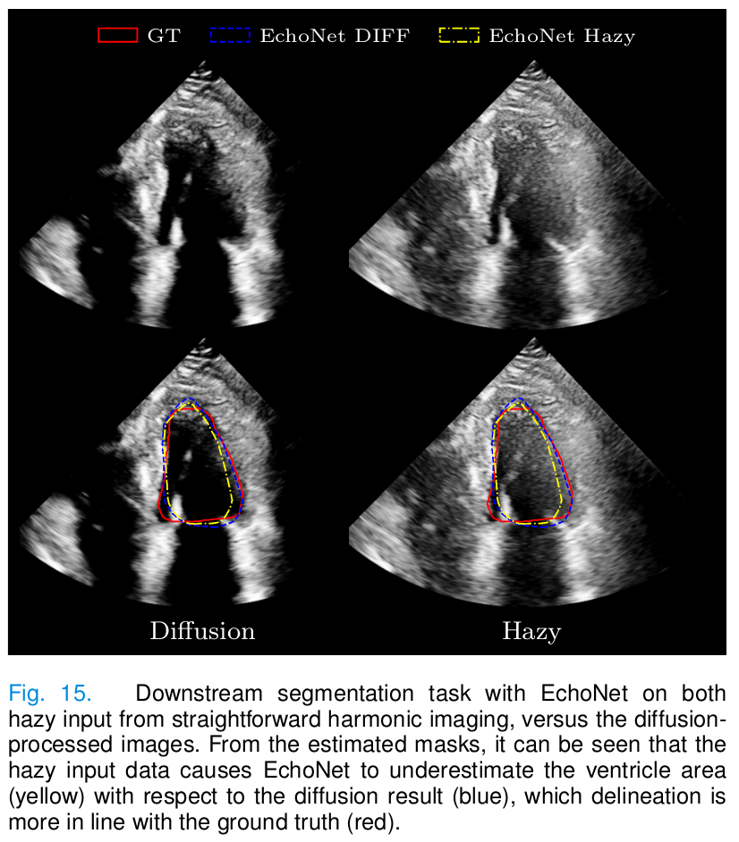
Downstream task: delineation of the left ventricle with a pretrained deep learning method (EchoNet).

Results

In vitro

The proposed method provides the reconstruction with better contrast and PSNR.
Baseline methods remove most of the haze but remove signal from low-level tissue.

In vivo

Diffusion provides the best gCNR scores.
BM3D removes too much tissue signal.
NCSNv2 fails to remove the haze due to domain shift.
The dehazing level is tunable via the parameter \(\gamma.\)
Images dehazed with diffusion allow for better left ventricle delineation.

Conclusions

Current dehazing techniques fail on several cases.
The authors proposed a dehazing framework using a joint posterior diffusion model by adapting techniques from deep generative modeling to the ultrasound (RF) domain.
The diffusion dehazing model provided improved images with respect to the baselines without the need of a paired supervised dataset.
The proposed posterior sampling method could be applied to other inverse problems in ultrasound other than dehazing.
The main limitation is that for now the inference cannot be performed real-time.