Diffusion Autoencoders: Toward a Meaningful and Decodable Representation
Highlights
- The denoising process is made easier and faster due to the semantic conditioning applied to the DDIM.
- The resulting representation is linear, semantically meaningful, and decodable.
- Code is available on this GitHub repo.
- A tuto is available on MONAI here.
Introduction
-
Autoencoders are useful for learning representations. On the contrary, DPM models can transform an input image into a latent variable yet they lack key features like semantics and disentanglement.
-
The proposed approach uses a learnable encoder to capture high-level semantics and a DPM for decoding and modeling variations.
-
Unlike other DPMs, DDIM introduces a non-Markovian reverse process while preserving DPM training objectives.
-
Conditioning DDIM on semantic information improves denoising efficiency and produces a linear, decodable, semantically meaningful representation. Also, due to the conditioning, the denoising becomes easier and faster.
-
To generate unconditional synthetic data, the authors used another DPM for the semantic subcode distribution.
Methods
Difference between DDPM and DDIM
DDPM and DDIM are both generative models with an identical forward process, leading them to share the same objective function. The difference between them is in the reverse process..
In DDPM, the reverse process is stochastic. The goal is to model the reverse diffusion process, starting from pure noise and progressively denoising it to generate a sample that resembles the original data.
1. Forward Process in DDPM:
\[q(x_t | x_{t-1}) = \mathcal{N}(x_t; \sqrt{1 - \beta_t} x_{t-1}, \beta_t I)\]2. Reverse Process in DDPM:
\[p_\theta(x_{t-1} | x_t) = \mathcal{N}(x_{t-1}; \mu_\theta(x_t, t), \Sigma_\theta(x_t, t))\]DDIM [1] introduces a non-Markovian modification to the reverse process, enabling deterministic sampling while preserving the training objective of DDPM.
1. Forward Process in DDIM:
\[q(x_t | x_0) = \mathcal{N}(x_t; \sqrt{\alpha_t} x_0, (1 - \alpha_t) I)\] \[\text{where } \alpha_t = \prod_{s=1}^{t} (1 - \beta_s)\]2. Reverse Process in DDIM:
\[x_{t-1} = \sqrt{\alpha_{t-1}} \left( \frac{x_t - \sqrt{1 - \alpha_t} \epsilon_\theta(x_t, t)}{\sqrt{\alpha_t}} \right) + \sqrt{1 - \alpha_{t-1}} \epsilon_\theta(x_t, t)\]Diffusion Autoencoders
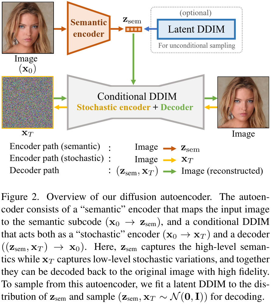
The authors introduce the semantic encoder (it learns to map an input image \(x_0\) to a semantically meaningful \(z_{\text{sem}}\)):
\[z_{\text{sem}} = \text{Enc}_\phi(x_0)\]and the decoder:
\[p_{\theta}(x_{t-1} | x_t, z_{\text{sem}})\]Here the decoder takes as input a latent variable \(z = (z_{\text{sem}}, x_T)\) (high-level “semantic” subcode \(z_{\text{sem}}\) and a low-level “stochastic” subcode \(x_T\)).
Diffusion-based Decoder
The conditional DDIM decoder proposed by the authors takes as input the pair \(z = (z_{\text{sem}}, x_T)\) to generate the output image. This decoder models \(p_{\theta}(x_{t-1} | x_t, z_{\text{sem}})\) to approximate the inference distribution \(q(x_{t-1} | x_t, x_0)\) using the following reverse generative process:
- Decoder:
- Training objective:
One benefit of conditioning DDIM with information-rich \(z_{\text{sem}}\) is more efficient denoising process.
The UNet they used is conditioned on \(t\) and \(z_{\text{sem}}\) using adaptive group normalization layers (AdaGN), which extend group normalization by applying channel-wise scaling and shifting to the normalized feature maps \(\mathbf{h} \in \mathbb{R}^{c \times h \times w}\) following the approach from Dhariwal et. al. [2]:
\[\text{AdaGN}(\mathbf{h}, t, z_{\text{sem}}) = z_s \left( t_s \text{GroupNorm}(\mathbf{h}) + t_b \right)\]where \(z_s \in \mathbb{R}^c = \text{Affine}(z_{\text{sem}})\)
and \((t_s, t_b) \in \mathbb{R}^{2 \times c} = \text{MLP}(\psi(t))\) is the output of a multilayer perceptron with a sinusoidal encoding function \(\psi\).
Sampling with diffusion autoencoders
Latent DDIM
Due to the conditioning of the decoder on \(z_{\text{sem}}\), diffusion autoencoders no longer function as generative models. To address this, the authors introduced a mechanism for sampling \(z_{\text{sem}} \in \mathbb{R}^{d}\) from the latent distribution.
They chose to fit another DDIM (called latent DDIM): \(p_{\omega}(z_{\text{sem}, t-1} | z_{\text{sem}, t})\)
to the latent distribution of \(z_{\text{sem}} = \text{Enc}_{\phi}(x_0), \quad x_0 \sim p(x_0)\)
They optimized
\[L_{\text{latent}} = \sum_{t=1}^{T} \mathbb{E}_{z_{\text{sem}}, \epsilon_t} \left[ \left\| \epsilon_{\omega}(z_{\text{sem}}, t) - \epsilon_t \right\|_1 \right]\]with
\[\epsilon_t \in \mathbb{R}^{d} \sim \mathcal{N}(0, I), z_{sem,t} = \sqrt{\alpha_t}z_{sem} + \sqrt{1 - \alpha_t}\epsilon_t\]For \(L_{\text{latent}}\), we empirically found that \(L_1\) works better than \(L_2\) loss
Training in practice
The authors used a deep MLPs (10-20 layers) with skip connections for the latent DDIM. They trained the semantic encoder (\(\phi\)) and the image decoder (\(\theta\)) until convergence. Then, they trained the latent DDIM (\(\omega\)) with the semantic encoder fixed.
In practice, the latent distribution modeled by the latent DDIM is first normalized to have zero mean and unit variance.
Unconditional sampling from a diffusion autoencoder is thus done by sampling \(z_{\text{sem}}\) from the latent DDIM and unnormalizing it, then sampling \(x_T \sim \mathcal{N}(0, I)\), and finally decoding \(z = (z_{\text{sem}}, x_T)\) using the decoder.
Results
High-level semantics and low-level stochastic variations
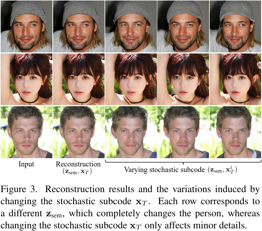
The figure below shows the variations when varying \(x_T\) with the same \(z_{\text{sem}}\) and the variations from different \(z_{\text{sem}}\) .
Semantically meaningful latent interpolation
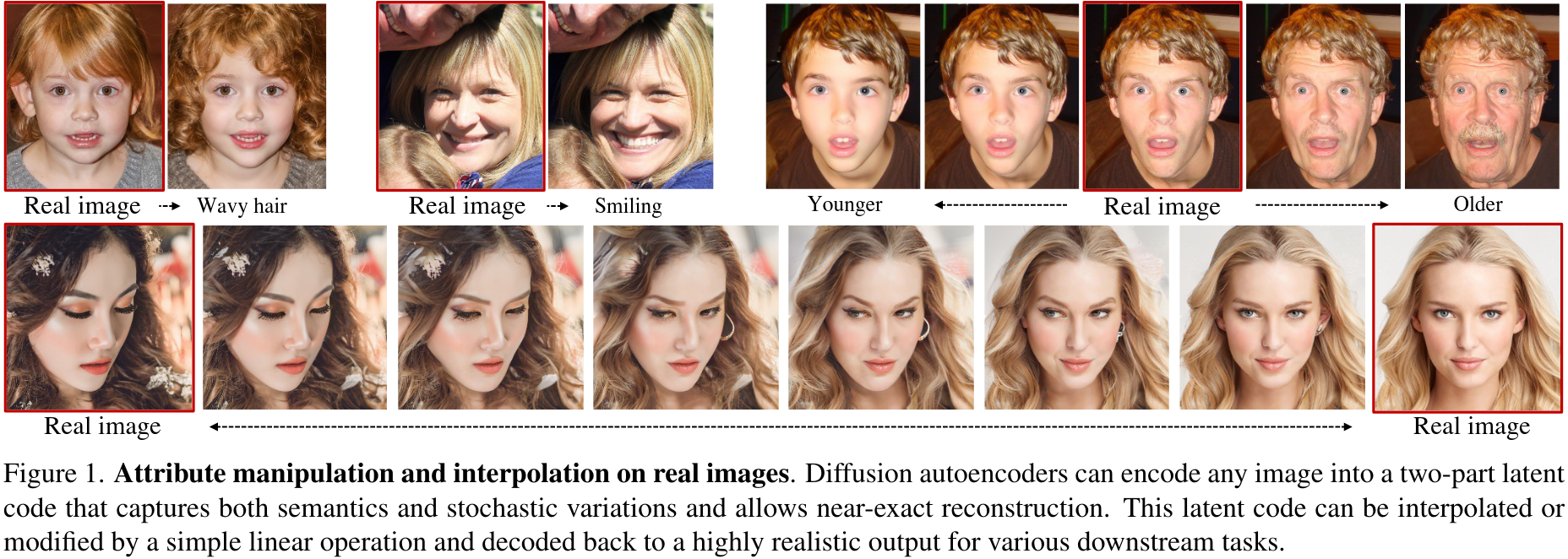
Here, they encode two input images (\(z_{\text{sem}}^{1}, x_T^1\)) and (\(z_{\text{sem}}^{2}, x_T^2\)) and applied a linear interpolation for \(z_{\text{sem}}\) and a spherical linear interpolation for \(x_T\).
Attribute manipulation on real images
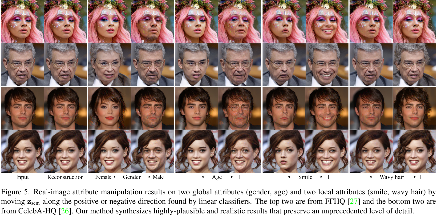
By moving the latent \(z_{\text{sem}}\) in a specific direction, the authors show that they can manipulate attribute images. These directions are found thanks to a linear classifier.
Quantitative results
Evaluation of the reconstruction quality:
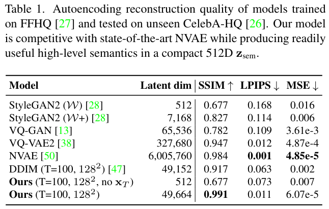
Evaluation of the reconstruction quality when only \(z_{\text{sem}}\) is encoded from the input but \(x_T\) is sampled from \(\mathcal{N}(0, I)\). They also evaluate the effects of varying the dimension of \(z_{\text{sem}}\):

Conclusion
In conclusion, this paper demonstrates the potential of leveraging DPMs for representation learning, aiming to extract meaningful and decodable representations of input images through an autoencoder framework.
References
[1] Song, J., Meng, C., Ermon, S. (ICLR 2021). Denoising diffusion implicit models.
[2] Dhariwal, P., & Nichol, A. (NeurIPS 2021). Diffusion models beat GANs on image synthesis.