Multi-Layers attention-based explainability via transformers for tabular data
Notes
- No code available :(
Highlights
- Investigate explainable models based on transformers for tabular data
- Use of knowledge distillation (master/student) to train a single head but multi-layers (blocks) transformer to facilitate explicability analysis
- Propose a graph-oriented explainability method based on the set of single head attention matrices
- Compare this approach to attention-, gradient-, and perturbation-based explainability methods
Introduction
- The field of explainable Artificial Intelligence is named XAI and has received increasing interest over the past decade
- XAI algorithms for DL can be organized into three major groups: perturbation-based, gradient-based, and, more recently, attention-based
- Transformers possess a built-in capability to provide explanations for their results via the analysis of attention matrices
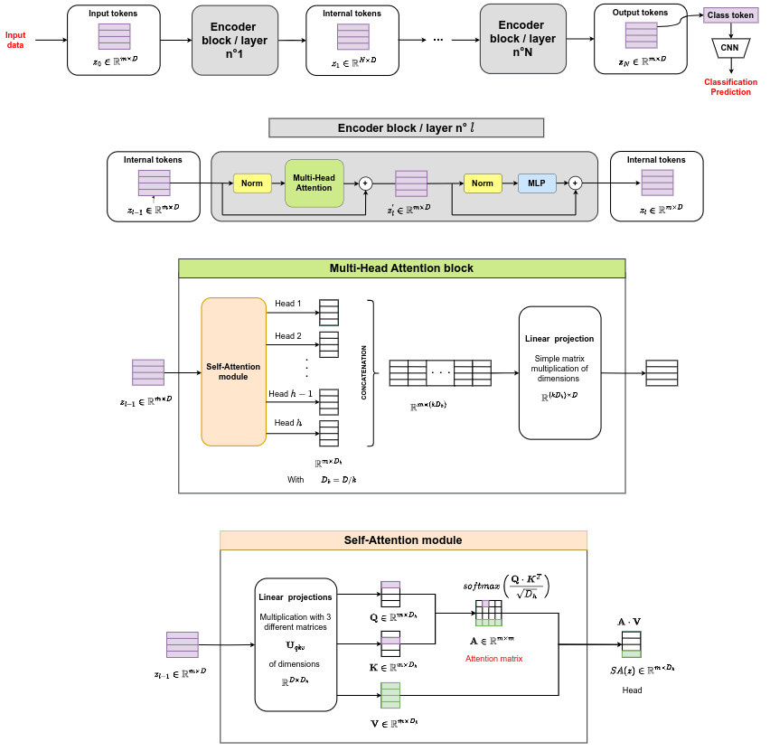
- A standard transformer encoder is composed of \(N \times h\) attention matrices, with \(N\) the number of blocks and \(h\) the number of heads per block
See the tutorial on transformers for more details.
Methodology
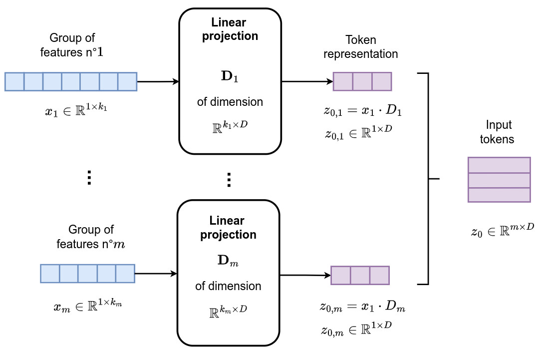
Groups of features
- Hypothesis 1: features within tabular data can often be grouped intuitively and naturally based on factors such as their source (e.g. sensors, monitoring systems, surveys) and type (e.g demographic, ordinal, or geospatial data)
- Hypothesis 2: given that tabular data does not provide sequential information, positional encoding is disabled
Knowledge distillation
- A full-capacity transformer (\(N\) blocks, \(h\) heads) is first trained for a classification task. This transformer is seen as a master transformer
- A student transformer is then trained to reproduce the same predictions as the ones from the master but using single heads (\(h=1\)) with more blocks (\(M>N\))
- The following student’s loss function is used
- The first term forces the student prediction \(\hat{y}_i\) to be close to the master’s \(y_i\)
- The second term forces the entropy of each attention matrix to be low => it forces the information contained in each attention matrix to be concentrated in a few cells => it forces the attention matrices to be sparse !
Multi-layer attention-based explainability
- Maps the attention matrices across encoder layers into a directed acyclic graph (DAG)
- The DAG is defined as \(D=(V,A)\), where \(V\) and \(A\) are the set of vertices and arcs that compose the graph \(D\)
- The vertices \(V= \bigcup_{l=0}^{M} \{ v^l_c \}\) correspond to groups of features, where \(c \in \{1,\cdots,m\}\)
- The arcs \(\left( v^{l-1}_{\hat{c}}, v^{l}_{\tilde{c}}\right) \in A\) correspond to attention values \(a^l_{\hat{c},\tilde{c}}\), where \(\hat{c}, \tilde{c} \in \{1,\cdots,m\}\)
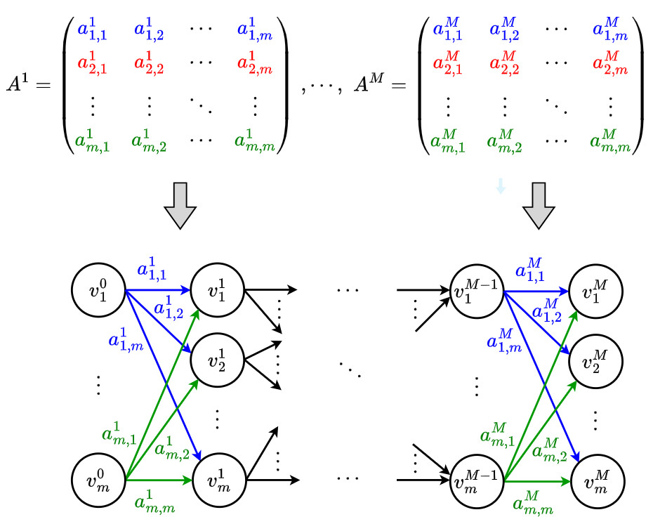
- The maximum probability path \(p\) is found using Dijkstra’s algorithm and is of the form \(p=\{ v^{0}_{i_0}, v^{1}_{i_1}, \cdots, v^{M}_{i_M} \}\)
- The arc cost is \(- \log\left( a^l_{j,k} \right)\) for \(a^l_{j,k} > 0\), yielding path cost \(- \log\left( \prod_{l=1}^{M} a^l_{i_{l-1},i_{l}} \right)\)
- The authors focus on the group of features corresponding to the most relevant input for the final prediction, i.e. group of features \(c=i_0\)
Explanations to the student’s predictions are provided by finding the most relevant group of features for the classification task, i.e. the group \(c=i_0\) corresponding to the first vertex \(v^0_{i_0}\) of the maximum probability path \(p\) in graph \(D\)
- A single group of features does not always provide all the relevant information to make a prediction
- Additional groups of features are ranked iteratively, i.e. in each iteration the starting point \(v^0_{i_0}\) of the previously found highest probability path is eliminated from the graph and Dijkstra’s algorithm is run again to search for the next highest probability path in \(D\)
- The best group is used most of the time in the experiments
Results
Classification datasets
- CT - Forest CoverType Dataset - Predict the most common cover type (3 class problem) for each 30m by 30m patch of forest. 425,000 samples were used for training and 53,000 for validation. 5 groups of features (general, distances, hillshades, wild areas, soil types) were used
- NI - Network Intrusion Dataset - Classification between bad connections (intrusions or attacks) and good connections. 1,000,000 samples were used for training and 75,000 for validation. 4 groups of features (basic, content, traffic, host) were used
- RW - Real-World Dataset - Binary classification problem. Tens of thousands of samples were used for training and validation. 8 groups of features were used. They had limited access to this private dataset and were unable to produce the same set of experiments as for the CT and NI dataset
Implementations
- Teacher network: \(N=2\) (number of blocs), \(h=4\) (number of heads per bloc), \(d=64\) (token size)
- Student network: \(M=4\) (number of blocs), \(h=1\) (number of heads per bloc), \(d=64\) (token size)
- Batch size of 128 and Adam optimizer
- \(\lambda_{CT} = 0.005\), \(\lambda_{NI} = 0.01\), and \(\lambda_{RW} = 0.9\)
- Each experiment was repeated five times for each CT and NI student and ten times for each RW student
Teacher/student classification performances
- Comparison with two standard machine learning methods: LightGBM and XGBoost
- Conceptual transformer is the student network
- The main goal is not to obtain the best performing model, but rather a competitive model that is better suited for explainability purposes

Table 1: Validation F1
- The performance of the student network has been validated as satisfactory and the multi-layer attention-based explanations are extracted for analysis
Explanation SOTA methods
-
Attention-based: Last-layer explainability (LL) The last layer’s self-attention head of the student’s encoder was analyzed. The best concept group to explain a given prediction was defined as that which corresponds to the highest attention value
-
Gradient-based: Saliency explainability (SA) The gradients of the loss function with respect to the input (concept groups) were computed. The best concept group to explain a given prediction was defined as the one that yields the largest mean absolute value
-
Perturbation-based: Shapley additive explanations (SH) The SHAP value of each feature was computed. The best concept group was defined as that with the largest mean absolute SHAP value
-
Attention head aggregation by averaging (AVG) This approach employs the teacher network instead of the distilled student and aggregates the heads from each layer by averaging them. The best concept group to explain a given prediction was defined as in the proposed MLA model (graph + Dijkstra algorithm)
Explanation distributions
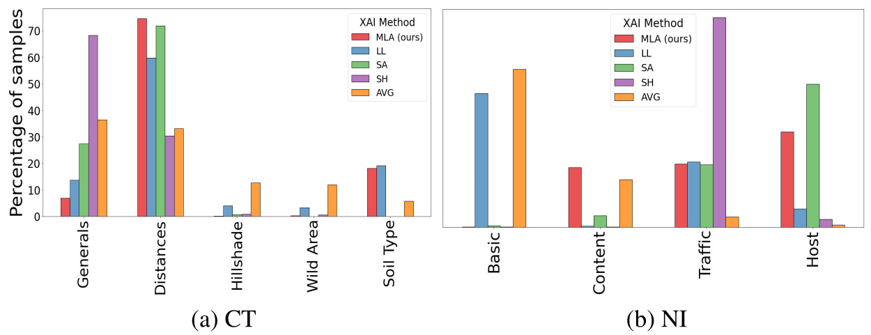
Figure 4 - Best concept group distribution per method
- For each method, the proportion of samples that considered each concept group to be the best is indicated
- For each dataset, the number of incorrectly classified samples is less than 5%, which has no impact on the overall distributions
- MLA appears to take more groups than SA and SH into account when identifying differences among samples
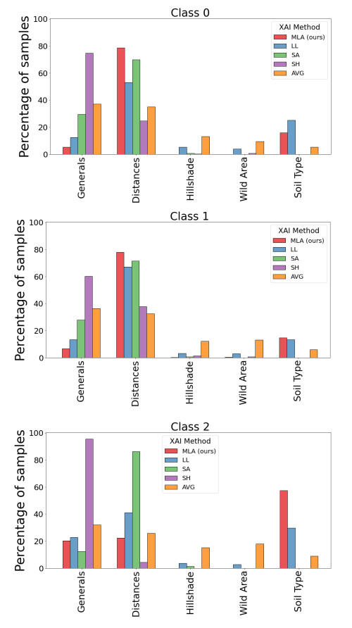
Figure 5 - CT’s best group of features per method by class
- Analysis of the proportion of samples that considered each concept group to be the best for CT, for each predicted class
- AVG demonstrates minimal to no alteration in its distribution according to the class, which seems strange
- MLA assigns explainability to three different concept groups for each class, with varying proportions depending on the class
- Strong alignment between LL and MLA behaviors
- Soil type seems to be a discriminating factor only for the LL and MLA methods

Figure 6 - CT’s Exploratory Data Analysis
- An Exploratory Data Analysis (EDA) was conducted on CT as a means to validate which features are most relevant for each class
- Soil Type does provide a clear differentiation between classes. All samples from Class 2 have soil types in {0, …, 9}, whereas samples from Class 0 do not have soil types lower than 9
- Even though the EDA clearly shows Soil Type concept group’s relevance for the classification task, only LL and MLA methods capture this information
Stability analysis
- The stability of the explanations is analyzed by quantifying the percentage of distinct runs that agree on the same explanation for each sample for MLA and LL methods

Figure 7 - Percentage of runs that agree on the best (1B) and two best (2B) context groups per method
- No real conclusion can be formulated from the 1B concept groups: for CT, we observe a better performance of MLA but larger variability than LL. On the other hand, the exact opposite can be said for RW, whereas both distributions seem to be identical for NI
- The use of 2B concept improves stability with averages of over 60% of agreement across runs, which remains relatively low !
- In the 2B concept case, the average model-to-model comparison seems to be dataset-dependent. However, MLA consistently shows lower variability than LL, making it more reliable and prone to provide robust and reliable explanations
Conclusions
- This paper presents a novel explainability method for tabular data that leverages transformer models and incorporates knowledge from the graph structure of attention matrices
- A method is proposed to identify the concept groups of input features that provide the most relevant information to make predictions
-
A comparison with existing explainability methods is performed
- Results show the interest of the graph method performed on the student network compared to the average method performed on the master network
- Unfortunately, no clear conclusions can be drawn from this paper
- The process of selecting the best group of features to make a predicition seems relatively simple