Rank-N-Contrast: Learning Continuous Representations for Regression
Code available on GitHub: https://github.com/kaiwenzha/Rank-N-Contrast
Highlights
-
A new framework, Rank-N-Contrast (RNC), that learns continuous representations for regression by contrasting samples against each other based on their rankings in the target space.
-
Experiments on five real-world regression datasets that highlight properties such as “better data efficiency, robustness to spurious targets and data corruptions, and generalization to distribution shifts”.
Introduction
Current approaches to deep regression fail to explicitly constrain representations to be regression-aware, i.e. to capture the continuous ordering of samples. The intuitive solution of directly predicting a scalar value and using a distance-based loss (e.g. \(L_1\) or \(L_2\) distance) between the predictions and target is still the most widely adopted approach for regression models. Because regressing precise values is a difficult problem, other baselines methods convert the regression into a classification problem by discretizing the target domain into small bins.
Across the different existing methods described above, the focus is on guiding the final predictions, i.e. the output of the prediction heads, in an end-to-end fashion. There are no explicit constraints on the learned representations themselves.
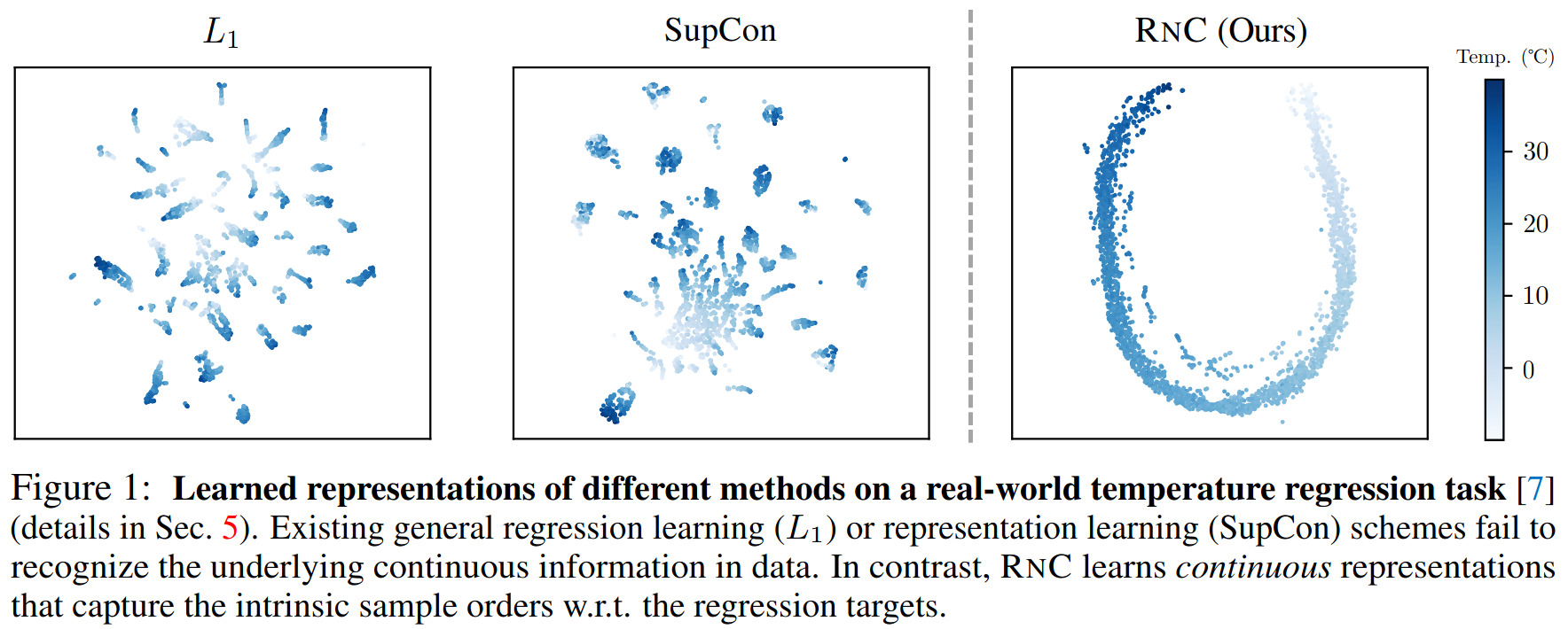
Figure 1. Representations learned on SkyFinder, a regression dataset for predicting weather temperature from webcam outdoor images.
Representation learning schemes for discrete tasks (e.g. contrastive learning1 for classification) and supervised contrastive learning (SupCon) have been widely successful. For example, SupCon “has been shown to outperform the conventional cross-entropy loss on multiple discrete classification tasks”. However, these approaches still overlook or straight up work against continuity in the data (see fig. 1).
Recap of representation learning schemes
Self-supervised Contrastive learning (SimCLR)
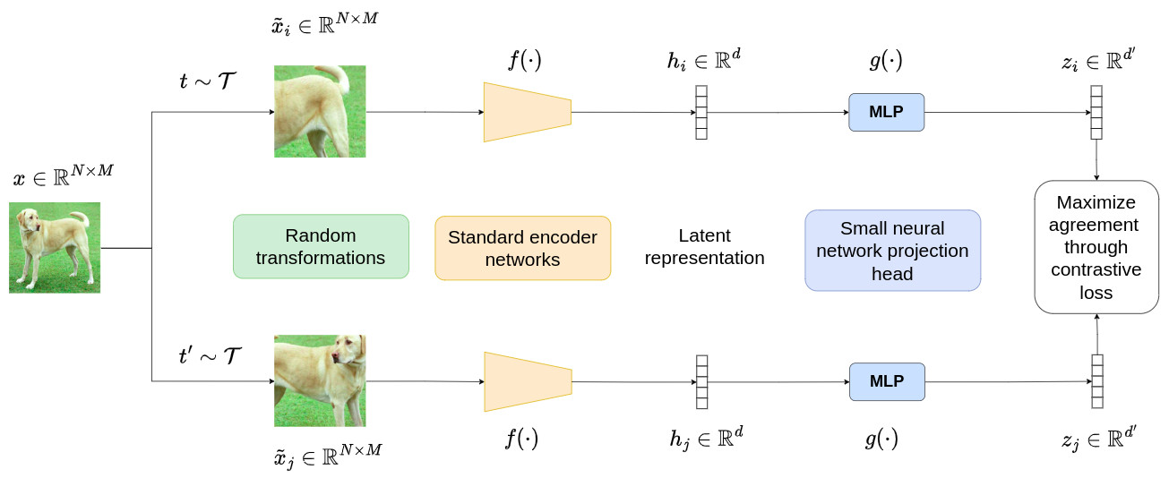
Popularized by SimCLR, the standard self-supervised contrastive learning pipeline applies label-invariant data augmentations to obtain two views of each sample. These views are considered positive pairs and are contrasted against the negative pairs which include views from other samples, i.e. their features are brought closer together, and farther away from other samples’ features.
Supervised Contrastive Learning (SupCon)2
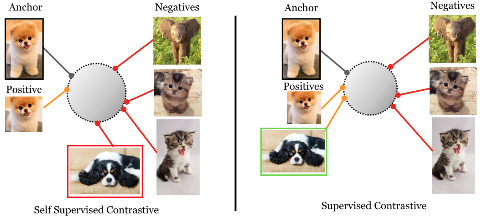
Compared to self-supervised contrastive learning, positive and negative pairs are determined by whether they belong to the same class, not whether they are different views of the same sample.
Methods
[The authors] propose the Rank-N-Contrast loss (LRNC), which ranks the samples in a batch according to their labels and then contrasts them against each other based on their relative rankings.
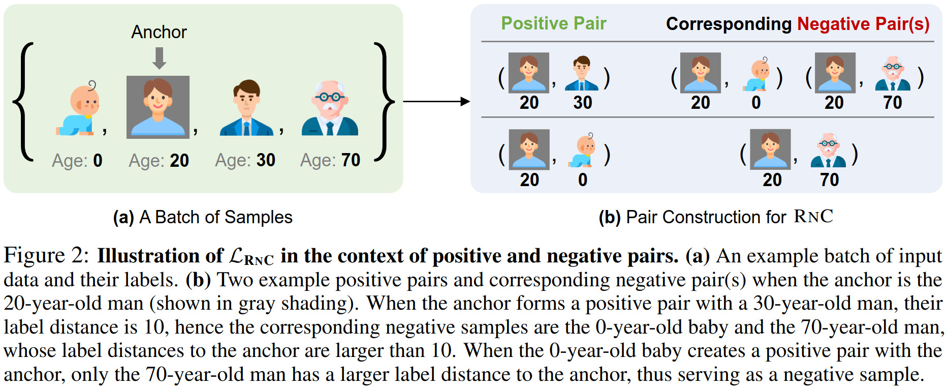
In mathematical terms, we can formulate this as:
\[S_{i,j} := \{ \mathbf{v}_k \mid k \ne i, d(\mathbf{\hat{y}}_i,\mathbf{\hat{y}}_k) \ge d(\mathbf{\hat{y}}_i,\mathbf{\hat{y}}_j) \}\]to denote the set of samples \(k\) that are of higher rank, i.e. further away, than sample \(j\) w.r.t. sample \(i\), with \(d(\cdot,\cdot)\) the distance between labels \(\mathbf{\hat{y}}\) (e.g. \(L_1\) distance).
Based on this ranking method, we can define a contrastive loss across a mini-batch of samples, which “align[s] the orders of features embeddings with their corresponding orders in the label space w.r.t. anchor \(i\)”:
\[\mathcal{L}_{\text{RNC}} = \underbrace{ \frac{1}{2N} \sum_{i=1}^{2N} }_{\text{Iterate over anchor } i} \quad \underbrace{ \frac{1}{2N-1} \sum_{j=1, j \ne i}^{2N} }_{\text{Iterate over ref. for negative pairs}} - \log \frac{ \overbrace{\exp(\text{sim}(\mathbf{v}_i,\mathbf{v}_j) / \tau)}^{\text{Bring closer samples } i \text{ and } j} } { \underbrace{\sum_{\mathbf{v}_k \in S_{i,j}} \exp(\text{sim}(\mathbf{v}_i,\mathbf{v}_k) / \tau)}_{\text{Push away samples of rank } \ge j} }.\]Here, \(\mathbf{v}\) represent the feature embeddings of samples learned by the model, \(\text{sim}(\cdot,\cdot)\) is the similarity between these features embeddings (e.g. negative \(L_2\) norm), and \(\tau\) is the standard softmax temperature hyperparameter.
Notably, [the] framework is orthogonal to existing regression methods, allowing for the use of any regression method to map the learned representation to the final prediction values.
Theoretical Analysis
The authors provide theoretical proofs that optimizing the contrastive problem, given how the positive and negative pairs are defined, “results in an ordered feature embedding that corresponds to the ordering of the labels”. However, I didn’t have time to properly dive into the maths.
Still, they insist on some important, and not necessarily intuitive, properties:
-
Scaling from batch to entire feature space: To achieve order between any triplet (\(i,j,k\)) of feature embeddings, is it necessary to optimize all (possible) batches to a sufficiently low loss? This would be practically infeasible, but the answer is no. The training “effectively [optimizes] the expectation of the loss over all possible random batches”, and “Markov’s inequality guarantees that when the expectation of the loss is optimized to be sufficiently low, the loss on any batch will be low enough with a high probability.”
-
Boosting of the final regression performance: How can ordering the feature embeddings help improve the final performance? Intuitively, “fitting an ordered feature embedding reduces the complexity of the regressor, which enables better generalization ability from training to testing. […] Specifically, if not constrained, the learned feature embeddings could capture spurious or easy-to-learn features that are not generalizable to the real continuous targets.”
-
Impact of data augmentation: In typical (self-supervised) contrastive learning techniques, obtaining multiple views through data augmentation is essential to the contrastive process. With RNC, other samples in the batch serve as anchors, i.e. positive pairs, so data augmentation is optional, just like for SupCon. It can help enhance model generalization, but it is no longer a critical component of the method.
Data
Experiments on five regression datasets across a variety of domains and structures of input data.
| Dataset | Prediction target | Input data | Nb of samples |
|---|---|---|---|
| AgeDB | Age (scalar) | 2D images of celebrities in-the-wild | 16,488 |
| IMBD-WIKI | Age (scalar) | 2D images of celebrities (posing) | 523,051 |
| TUAB | Brain-age (scalar) | 21-channel EEG signals | 1,385 |
| MPIIFaceGaze | Gaze direction (2D vector) | 2D images collected during everyday laptop use | 213,569 (from 15 participants) |
| SkyFinder | Temperature (scalar) | 2D images from outdoor webcams | 35,417 |
Results
Experimental setup
-
ResNet-18 as the main backbone for AgeDB, IMDB-WIKI, MPIIFaceGaze, and SkyFinder. Appendix shows consistent results with a ResNet-50 backbone (but not more variety of architectures);
-
For the MPIIFaceGaze dataset, since the target is not a scalar, angular distance was used as label distance, instead of negative \(L_2\) norm.
Comparisons to regression and representation learning methods
Comparisons to seven generic regression methods, which can be grouped like follows:
- Error-based loss function: \(L_1\), MSE, and HUBER;
- Discretization of the regression range in pre-defined bins + classification: DEX, DLDL-V2;
- Multiple ordered thresholds for each label dimension + one binary classifier per threshold: OR, CORN.
In our comparison, we first train the encoder with the proposed \(\mathcal{L}_{\text{RNC}}\). We then freeze the encoder and train a predictor on top of it using each of the baseline methods. The original baseline without the RNC representation is then compared to that with RNC.
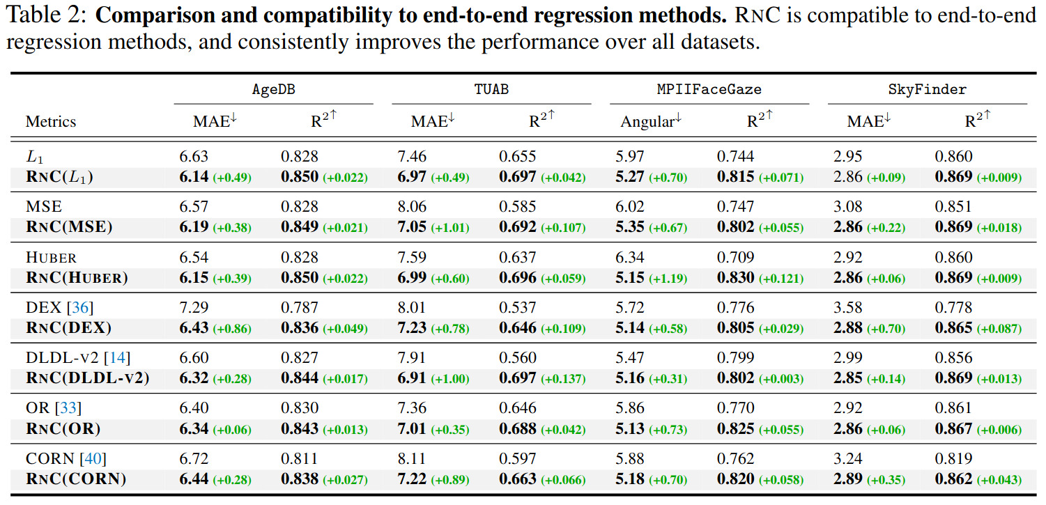
A comparison to the representation learning methods, both classification-oriented (e.g. SimCLR, Dino, SupCon) and regression-based (e.g. ordinal entropy) is available in the paper, showing that RNC outperforms all other approaches.
Robustness and generalizability properties
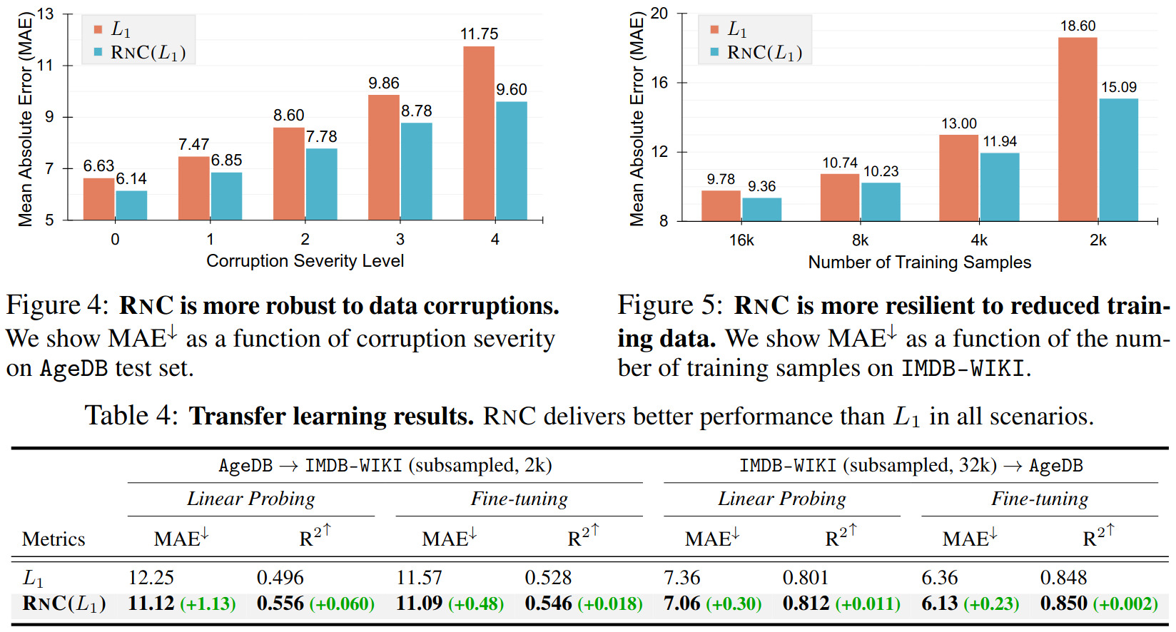
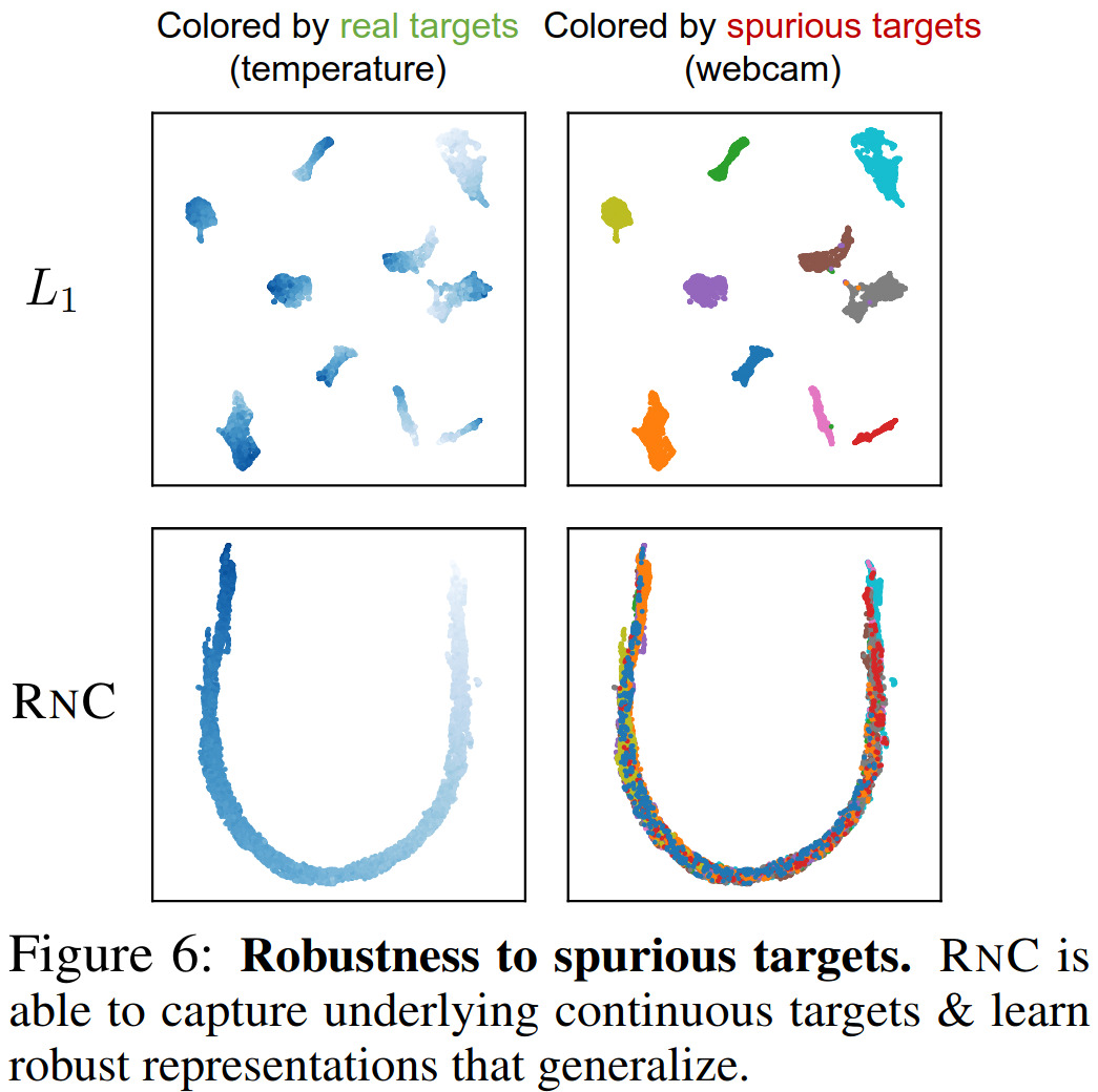
An additional study on zero-shot generalization to unseen regression target ranges is provided in the paper, showing that RNC performs better than the \(L_1\) norm.
Ablation studies

Editorial comments
-
Contrasting samples by ranking their scalar values, instead of trying to correlate to the values directly, reminds me of the AR-VAE’s attribute regularization loss3, which I’ve found works well in practice. The authors expressed my own intuition for why it helps in their answer to the question on boosting performance in the theoretical analysis section;
-
This paper mostly focused on continuous scalar targets, but the experiment on MPIIFaceGaze shows that the method can generalize to multidimensional continuous vectors, as long as their is an appropriate distance measure for the task. However, I would be curious to see visualization of the feature embeddings in a multidimensional setting.
References
-
Tutorial on contrastive learning: https://creatis-myriad.github.io/tutorials/2022-06-20-tutorial_contrastive_learning.html ↩
-
Paper that popularized supervised contrastive learning: P. Khosla et al., Supervised Contrastive Learning, NeurIPS 2020 ↩
-
Review of AR-VAE: https://creatis-myriad.github.io/2023/03/02/AttributeRegularizedVAE.html ↩